2021년 5월 27일 목요일

딥러닝 모델의 Convolution 필터 동작 구조

이 글은 딥러닝 모델의 컨볼루션 필터의 동작 구조를 설명한 것이다.

머리말
CNN(convolutional neural network)은 특정 방향의 모서리(edge)를 강조하는 edge detection, 상세를 강조해 blurring을 제거해주는 sharpness filter 등의 다양한 필터를 사용해 특징을 추출한다. 이를 컨볼루션 필터라 한다.

많은 컨볼루션 아키텍처는 채널 RGB의 입력 이미지를 일련의 내부 필터에 매핑하는 컨볼 루션으로 시작한다. 가장 많이 사용되는 딥러닝 프레임 워크에서 다음 코드는 많이 보여진다.

out_1 = Conv2d (input = image, filter = 32, kernel_size = (3,3), strides = (1,1))
relu_out = relu (out_1)
pool_out = MaxPool (relu_out, kernel_size = (2,2), strides = 2)

위의 결과는 32란 값은 일련의 필터들 갯수라는 것을 알고 있다. 다음 그림은 이 계산과정을 나타낸다.


1 단계 각 필터(filter-1, filter-2,… 등)가 3개 컨볼루션 커널(Wt-R, Wt-G 및 Wt-B)에 적용된다. 순방향 전파 중에 이미지의 R, G 및 B 픽셀 값이 각각 Wt-R, Wt-G 및 Wt-B 필터 커널에 곱해져 활성화 맵을 생성한다. 그런 다음 세 커널의 출력을 추가하여 필터 당 하나의 활성화 맵을 생성한다. 이러한 활성화는 ReLu 함수에 적용되고, 최대 풀링 계층을 통해 실행된다. 

컨볼루션 필터는 다음과 같은 종류가 있다. 
  • 1 차원 데이터에 대한 1D 컨볼 루션 (시간)
  • 2 차원 데이터에 대한 2D 컨볼 루션 (높이 및 너비)
  • 3 차원 데이터에 대한 3D 컨볼 루션 (높이, 너비 및 깊이)
Conv1D 
아이스크림 판매 예측의 경우를 보겠다. 입력은 시간적 차원에 따라 매일 간격으로 정의 될 수 있다. 제품 가격, 마케팅 지출, 외부 온도 및 주말인지 여부에 대한 정규화된 값을 가질 수 있다. 아래 경우는 총 4 개의 채널을 가진다. 
6 개의 시간에 걸쳐 4 개 채널이 있는 입력 배열

입력 데이터가 2차원처럼 보이지만, 차원 중 하나만 공간적이다. 4개 변수 (A, B, C, D)는 무작위 순서로 시작하면 A & B, B & C 및 C & D간에 유사한 공간 관계를 찾을 수 없다.
이러한 이유로 다중 채널 시간 데이터로 작업할 때는 1D Convolution을 사용하는 것이 가장 좋다. 
1x4 출력위해 4x6 입력 행렬에 적용 커널크기 3의 1D컨볼루션

컨볼루션 레이어에 입력 데이터를 필터가 순회하며 합성곱을 통해서 만든 출력을 피처맵(Feature Map) 또는 액티베이션 맵(Activation Map)이라고 한다. 액티베이션 맵은 피처맵 행렬에 활성 함수를 적용한 결과이다. 

앞의 과정은 다음 코드로 표현할 수 있다.

# input_data.shape는 (4, 6) 
# kernel.shape는 (4, 3)
conv = Conv1D (channels = 1, kernel_size = 3)
output_data = apply_conv (input_data, kernel, conv) 
print (output_data)
# [[[24. 25. 22. 15.]]] 

Conv2D 
컬러 이미지는 다중 채널 공간 데이터의 좋은 예이다. 다음 그림에서 각 위치 색상을 나타내는 3개의 채널이 있다. 
3 개 채널 표현

3x3 커널을 정의하더라도 3개 입력채널이 있어, 초기화될 때 커널의 실제 크기는 3x3x3이 될 것이다. 
3x3 출력 위해 크기 5x5인 3채널 RGB 입력에 3x3 커널을 적용한 2D 컨볼루션

# input_data.shape는 (3, 5, 5) 
# kernel.shape는 (3, 3, 3).
conv = Conv2D (channels = 1, kernel_size = (3,3))
output_data = apply_conv (input_data, 커널, conv) 
print (output_data)
# [[[[19. 13. 15.] 
# [28. 16. 20.] 
# [23. 18. 25.]]]] 
# <NDArray 1x1x3x3 @cpu (0)>

다중출력채널 컨볼루션
하나의 컨볼루션 필터만 사용하면, 너무 한정된 특징만 추출될 수 있다. 그러므로, 출력채널이 다중인 컨볼루션을 다음과 같이 사용할 수 있다.
컨볼루션 계층 4개 커널 출력 최대화

다중출력채널은 학습 시 주어진 클래스에 대한 이미지의 서로 다른 엣지, 색깔, 블롭(blob) 등에 활성화되는 필터들을 의미한다. 이를 입력 데이터와 계산하면, 결국 깊이값으로 표현되기 때문에, 깊이컬럼(depth column)이라 부르기도 한다.

여러 출력채널을 추가하면, 다음과 같이 계산된다. 
4x4 출력위해 크기 3커널 4개 1x6 입력 행렬에 적용한 1D컨볼루션

코드로 나타내면 다음과 같다.
# input_data.shape는 (1, 6) 
# kernel.shape는 (4, 1, 3)
conv = Conv2D (channels = 4, kernel_size = (3,3))
output_data = apply_conv (input_data, kernel, conv) 
print (output_data)
# [[[5. 6. 7. 2.] 
# [6. 6. 0. 2.] 
# [9. 12. 10. 3.] 
# [10. 6. 5. 5.]]] 

2021년 5월 24일 월요일

패션 이미지 데이터 활용 PyTorch 기반 모델 훈련 및 예측 방법

이 글은 패션 이미지 데이터를 활용한 PyTorch 기반 모델 훈련 및 예측 방법을 간단히 나눔한다. 
파이토치(Pytorch)는 파이썬기반 오픈 소스 머신러닝 라이브러리로 페이스북 인공지능 연구소에 의해 개발되었다. 파이토치는 NVIDIA의 GPU로 병렬처리가 가능해, 높은 실행 성능을 가진다.  토치 사용방법은 Keras와 유사하나, 좀 더 간단히 신경망을 정의하고, 지원되는 유틸리티 사용이 편리하다. 이 글은 패션 이미지를 MNIST처럼 공유한 데이터를 사용해 학습 및 예측을 진행하고, 이를 설명한다. 

PyTorch 설치 방법
여러가지 설치 방법이 있으나, 여기서는 anaconda를 사용하기로 한다. pytorch 설치 전에 아래를 참고해, NVIDIA DRIVER, CUDA, 텐서플로우 등을 설치해야 한다. 참고로, 운영체제 환경에 따라 설치 방법은 약간 다를 수 있다. 
아래 명령으로 토치를 설치한다.
conda install -c pytorch pytorch

참고로, CUDA 버전에 따라 설치되는 패키지 버전 의존성이 달라져 에러가 발생할 수도 있다. 이 경우는 정답이 없어, 구글링하면서 솔류션을 찾아야 한다.

FashionMNIST 학습 및 예측
FashionMNIST는 아래와 같은 패션 데이터이다. 
이 패션 데이터셋은 Zalando의 패션 작품 이미지로 훈련용 60,000개, 테스트용 10,000개 이미지를 제공한다. 각 이미지는 28x28 회색 이미지이며, 각 이미지별 라벨(label)이 저장되어 있다. 
라벨은 다음과 같다. 
Label Description
0         T-shirt/top
1         Trouser
2         Pullover
3         Dress
4         Coat
5         Sandal
6         Shirt
7         Sneaker
8         Bag
9         Ankle boot

아래 코드를 입력하고, 실행해본다.

# 라이브러리 임포트
import torch
from torch import nn
from torch.utils.data import DataLoader
from torchvision import datasets
from torchvision.transforms import ToTensor, Lambda, Compose
import matplotlib.pyplot as plt

# 패션 MNIST 훈련용 데이터셋을 다운로드한다.
training_data = datasets.FashionMNIST(
    root="data",
    train=True,
    download=True,
    transform=ToTensor(),
)

# 테스트 데이터를 다운로드한다.
test_data = datasets.FashionMNIST(
    root="data",
    train=False,
    download=True,
    transform=ToTensor(),
)

batch_size = 64  # 배치크기 설정

# 데이터 로더 생성
train_dataloader = DataLoader(training_data, batch_size=batch_size)
test_dataloader = DataLoader(test_data, batch_size=batch_size)

for X, y in test_dataloader:
    print("Shape of X [N, C, H, W]: ", X.shape)
    print("Shape of y: ", y.shape, y.dtype)
    break

# 학습용 디바이스 정보 획득
device = "cuda" if torch.cuda.is_available() else "cpu"
print("Using {} device".format(device))

# 모델 정의
class NeuralNetwork(nn.Module):
    def __init__(self):
        super(NeuralNetwork, self).__init__()
        self.flatten = nn.Flatten()
        self.linear_relu_stack = nn.Sequential(
            nn.Linear(28*28, 512),
            nn.ReLU(),
            nn.Linear(512, 512),
            nn.ReLU(),
            nn.Linear(512, 10),
            nn.ReLU()
        )

    def forward(self, x):
        x = self.flatten(x)
        logits = self.linear_relu_stack(x)
        return logits

# 모델 학습을 위한 디바이스 설정
model = NeuralNetwork().to(device)
print(model)

# 모델 학습 솔류션 수렴을 위한 최적화 모델 정의
loss_fn = nn.CrossEntropyLoss()
optimizer = torch.optim.SGD(model.parameters(), lr=1e-3)

# 훈련 함수 정의
def train(dataloader, model, loss_fn, optimizer):
    size = len(dataloader.dataset)
    for batch, (X, y) in enumerate(dataloader):
        X, y = X.to(device), y.to(device)

        # Compute prediction error
        pred = model(X)
        loss = loss_fn(pred, y)

        # Backpropagation
        optimizer.zero_grad()
        loss.backward()
        optimizer.step()

        if batch % 100 == 0:
            loss, current = loss.item(), batch * len(X)
            print(f"loss: {loss:>7f}  [{current:>5d}/{size:>5d}]")

# 테스트 함수 정의
def test(dataloader, model):
    size = len(dataloader.dataset)
    model.eval()
    test_loss, correct = 0, 0
    with torch.no_grad():
        for X, y in dataloader:
            X, y = X.to(device), y.to(device)
            pred = model(X)
            test_loss += loss_fn(pred, y).item()
            correct += (pred.argmax(1) == y).type(torch.float).sum().item()
    test_loss /= size
    correct /= size
    print(f"Test Error: \n Accuracy: {(100*correct):>0.1f}%, Avg loss: {test_loss:>8f} \n")

epochs = 10  # 학습을 원하는 만큼 수정요
for t in range(epochs):
    print(f"Epoch {t+1}\n-------------------------------")
    train(train_dataloader, model, loss_fn, optimizer)
    test(test_dataloader, model)
print("Done!")

# 모델 학습 가중치 파일 저장
torch.save(model.state_dict(), "model.pth")
print("Saved PyTorch Model State to model.pth")

# 가중치 파일을 통한 모델 로드
model = NeuralNetwork()
model.load_state_dict(torch.load("model.pth"))

# 예측을 위한 클래스 정의
classes = [
    "T-shirt/top",
    "Trouser",
    "Pullover",
    "Dress",
    "Coat",
    "Sandal",
    "Shirt",
    "Sneaker",
    "Bag",
    "Ankle boot",
]

# 모델 평가
model.eval()
x, y = test_data[0][0], test_data[0][1]
with torch.no_grad():
    pred = model(x)  # 패션 MNIST 데이터 입력 후 예측
    predicted, actual = classes[pred[0].argmax(0)], classes[y]
    print(f'Predicted: "{predicted}", Actual: "{actual}"')

실행 결과는 다음과 같다.
/home/ktw/anaconda3/envs/pytorch/bin/python /home/ktw/.local/share/JetBrains/Toolbox/apps/PyCharm-C/ch-0/211.6693.115/plugins/python-ce/helpers/pydev/pydevd.py --multiproc --qt-support=auto --client 127.0.0.1 --port 39301 --file /home/ktw/Projects/pytorch/MNIST.py
Connected to pydev debugger (build 211.6693.115)
Backend Qt5Agg is interactive backend. Turning interactive mode on.
Shape of X [N, C, H, W]:  torch.Size([64, 1, 28, 28])
Shape of y:  torch.Size([64]) torch.int64
Using cuda device
NeuralNetwork(
  (flatten): Flatten(start_dim=1, end_dim=-1)
  (linear_relu_stack): Sequential(
    (0): Linear(in_features=784, out_features=512, bias=True)
    (1): ReLU()
    (2): Linear(in_features=512, out_features=512, bias=True)
    (3): ReLU()
    (4): Linear(in_features=512, out_features=10, bias=True)
    (5): ReLU()
  )
)
Epoch 1
-------------------------------
loss: 2.299011  [    0/60000]
loss: 2.295951  [ 6400/60000]
loss: 2.283560  [12800/60000]
loss: 2.278397  [19200/60000]
loss: 2.284869  [25600/60000]
loss: 2.267760  [32000/60000]
loss: 2.266866  [38400/60000]
loss: 2.257998  [44800/60000]
loss: 2.237380  [51200/60000]
loss: 2.209423  [57600/60000]
Test Error: 
 Accuracy: 41.4%, Avg loss: 0.034879 

...
est Error: 
 Accuracy: 57.0%, Avg loss: 0.022959 

Done!
Saved PyTorch Model State to model.pth
Predicted: "Sneaker", Actual: "Ankle boot"

이제 학습 반복 세대를 높여서 실행해보자. 세대를 10으로 수정한 후 loss는 0.018335로 줄었음을 확인할 수 있다.

파이토치 기능 및 모델구조 설명
토치는 데이터 로딩 작업을 위해, torch.utils.data.DataLoader, torch.utils.data.Dataset을 제공한다. torchvision.datasets 모듈은 CIFAR, COCO 등 유명한 데이터셋 로딩을 지원한다. 

앞의 소스에서 배치 크기는 64이므로, 데이터로더의 iterator는 64개의 이미지와 레이블을 반환하게 된다. 

모델 정의는 다음과 같다. 
class NeuralNetwork(nn.Module):
    def __init__(self):
        super(NeuralNetwork, self).__init__()
        self.flatten = nn.Flatten()
        self.linear_relu_stack = nn.Sequential(
            nn.Linear(28*28, 512),
            nn.ReLU(),
            nn.Linear(512, 512),
            nn.ReLU(),
            nn.Linear(512, 10),
            nn.ReLU()
        )

    def forward(self, x):
        x = self.flatten(x)
        logits = self.linear_relu_stack(x)
        return logits

토치의 상위 클래스, nn.Module을 파생받은 NeuralNetwork 클래스를 정의해야 한다(Torch.NN 참고).

생성자에서 모델을 정의한다. nn은 신경망 구조를 제공한다. nn.ReLU는 비선형 학습 활성화 함수를 정의한다. flatten은 주어진 2차원 벡터 이미지를 1차원으로 벡터로 변환한다. 

nn.Sequential은 정의된 순서대로 데이터가 전달되도록 하는 컨테이너이다. 이 컨테이너에 신경망 구조를 순서대로 정의하면 된다. 모델링된 결과는 다음과 같다. 28x28 이미지(784 픽셀)는 Linear 레이어로 입력되어, 512 출력노드로 맵핑된다. 이 레이어의 출력값은 ReLU로 전달되고, 다시 Linear 레이어로 512 출력노드로 맵핑되어 ReLU로 변환된다. 이 결과는 다시 10개의 출력노드를 가진 Linear 레이어로 맵핑되고 ReLU로 변환된다. 

NeuralNetwork(
  (flatten): Flatten(start_dim=1, end_dim=-1)
  (linear_relu_stack): Sequential(
    (0): Linear(in_features=784, out_features=512, bias=True)
    (1): ReLU()
    (2): Linear(in_features=512, out_features=512, bias=True)
    (3): ReLU()
    (4): Linear(in_features=512, out_features=10, bias=True)
    (5): ReLU()
  )
)

역전파 알고리즘 함수는 토치에서 train의 forward함수를 이용해 자동으로 생성해준다.
역전파 알고리즘은 신경망의 입력층과 출력층의 차이를 조정하기 위해, 가중치를 얼마나 보정해야 하는 지를 계산한다. 이 보정치는 손실함수의 기울기값이라고 말하며, 이는 다음 그림에서 신경망 가중치와 바이어스를 기울기 값으로 수정할때 사용된다. 손실함수는 계산된 결과와 목표값의 차이를 계산하여, 이 차이값을 최소화할 때 사용된다.
모델 훈련은 이러한 과정을 반복해 가중치와 바이어스를 조정하는 수치 계산 과정일 뿐이다. 

앞의 소스에서는 학습 파라메터인 파이퍼 파라메터를 다음과 같이 설정했었다. 
learning_rate = 1e-3
batch_size = 64
epochs = 5

여기서 learning_rate는 옵티마이저에 설정되는 학습률이다. 

옵티마이저는 각 학습 단계에서 모델 오류를 줄이기 위해 모델 손실값을 조정해 나간다. SDG는 확률기반 경사 하강법이며, 토치에는 이외 다양한 최적화 함수가 있다. 모델의 파라메터를 통해 최적화 함수는 모델 구조, 파라메터, 역전파 함수를 얻어 이를 최적화할 때 사용한다.
optimizer = torch.optim.SGD(model.parameters(), lr=learning_rate)

결국, 다음과 같이 앞에서 정의한 데이터 로딩 방법, 모델, 손실 함수, 최적화 함수를 이용해 세대별로 반복 학습을 하게 된다.
for t in range(epochs):
    print(f"Epoch {t+1}\n-------------------------------")
    train(train_dataloader, model, loss_fn, optimizer)
    test(test_dataloader, model)

훈련된 모델은 파일로 저장해 필요할 때 로딩해 사용할 수 있다. ONNX(Open Neural Network Exchange) 로딩 및 저장도 함께 제공한다.

모델 구조 수정 후 결과 비교
모델 구조를 수정해 결과를 확인해 보자. 참고로, 원래 소스 결과는 5세대 훈련 시  Accuracy: 57.0%, Avg loss: 0.022959 였다. 

1. 2개 은닉층
NeuralNetwork(
  (flatten): Flatten(start_dim=1, end_dim=-1)
  (linear_relu_stack): Sequential(
    (0): Linear(in_features=784, out_features=512, bias=True)
    (1): ReLU()
    (2): Linear(in_features=512, out_features=10, bias=True)
    (3): ReLU()
  )
)

Test Error: 
 Accuracy: 33.4%, Avg loss: 0.030179 

Done!
Saved PyTorch Model State to model.pth
Predicted: "Ankle boot", Actual: "Ankle boot"

2. 4개 은닉층
NeuralNetwork(
  (flatten): Flatten(start_dim=1, end_dim=-1)
  (linear_relu_stack): Sequential(
    (0): Linear(in_features=784, out_features=512, bias=True)
    (1): ReLU()
    (2): Linear(in_features=512, out_features=512, bias=True)
    (3): ReLU()
    (4): Linear(in_features=512, out_features=512, bias=True)
    (5): ReLU()
    (6): Linear(in_features=512, out_features=10, bias=True)
    (7): ReLU()
  )
)

Test Error: 
 Accuracy: 38.2%, Avg loss: 0.032565 

Done!
Saved PyTorch Model State to model.pth
Predicted: "Ankle boot", Actual: "Ankle boot"

3. 4개 은닉층에서 입출력을 512-256으로 매핑.
NeuralNetwork(
  (flatten): Flatten(start_dim=1, end_dim=-1)
  (linear_relu_stack): Sequential(
    (0): Linear(in_features=784, out_features=512, bias=True)
    (1): ReLU()
    (2): Linear(in_features=512, out_features=512, bias=True)
    (3): ReLU()
    (4): Linear(in_features=512, out_features=256, bias=True)
    (5): ReLU()
    (6): Linear(in_features=256, out_features=10, bias=True)
    (7): ReLU()
  )
)

Test Error: 
 Accuracy: 39.7%, Avg loss: 0.032889 

Done!
Saved PyTorch Model State to model.pth
Predicted: "Ankle boot", Actual: "Ankle boot"

결과와 같이 모델 구조에 따라 정확도 및 손실률이 달라진다. 이 모델은 CNN을 사용하지 않았다. 다음과 같이 CNN 모델을 사용할 경우, 정확도는 매우 높아진다. 

CNN 모델은 다음과 같이 정의한다.
x = Image(28 * 28 * 1)  # 그레이컬러 입력채널 1개, 이미지 크기 28 x 28
x = x * Conv2d(1, 8, 3)       # 입력채널 1개, 출력(필터)채널 8개, 커널크기 3
x = ReLu(x)
x = Pooling(x)
x = x* Conv2d(8, 16, 3)     # 입력채널 8개, 출력채널 16개, 커널크기 3
x = ReLu(x)
x = Pooling(x)
x = Reshape(x, -1, 7 * 7 * 16)
x = Dropout(ReLu(Linear(x, 28 * 28, 16 * 16))) # 입력 이미지 28 x 28, 출력 256
x = Dropout(ReLu(Linear(x, 16 * 16, 128)))
x = Dropout(ReLu(Linear(x, 128, 8 * 8)))
x = Linear(x, 8 * 8, 10)
 
코드 구현은 다음과 같다. 
class Net(nn.Module):
    def __init__(self):
        super(Net, self).__init__()
        # convolutional layers
        self.conv1 = nn.Conv2d(1, 8, 3, padding=1)  
        self.conv2 = nn.Conv2d(8, 16, 3, padding=1)
        # linear layers
        self.fc1 = nn.Linear(784, 256)
        self.fc2 = nn.Linear(256, 128)
        self.fc3 = nn.Linear(128, 64)
        self.fc4 = nn.Linear(64, 10)
        # dropout
        self.dropout = nn.Dropout(p=0.2)
        # max pooling
        self.pool = nn.MaxPool2d(2, 2)

    def forward(self, x):
        # convolutional layers with ReLU and pooling
        x = self.pool(F.relu(self.conv1(x)))
        x = self.pool(F.relu(self.conv2(x)))
        # flattening the image
        x = x.view(-1, 7 * 7 * 16) # reshape
        # linear layers
        x = self.dropout(F.relu(self.fc1(x)))
        x = self.dropout(F.relu(self.fc2(x)))
        x = self.dropout(F.relu(self.fc3(x)))
        x = self.fc4(x)
        return x

이 경우, 정확도는 평균 77.31%로 높아진다. 레이어가 깊다고 정확도가 높아지는 것은 아니다. 실제 Conv2d(64, 32) 층을 하나 더 추가하고 학습하면 정확도가 67.19%로 오히려 떨어지는 현상을 볼 수 있다. 

다음과 같이 레이어를 하나 더 줄이고 테스트하면 오히려 정확도가 79.98%로 높아진다. 정확도는 학습 데이터 수, 품질, 학습 횟수 등 모델 구조 이외 다른 요소들도 영향을 주므로, 이런 부분은 경험적으로 모델을 설계해야 한다.

lass Net(nn.Module):
    def __init__(self):
        super(Net, self).__init__()
        # convolutional layers
        self.conv1 = nn.Conv2d(1, 8, 3, padding=1)
        self.conv2 = nn.Conv2d(8, 16, 3, padding=1)
        # linear layers
        self.fc1 = nn.Linear(784, 256)
        self.fc2 = nn.Linear(256, 96)
        self.fc3 = nn.Linear(96, 10)
        # dropout
        self.dropout = nn.Dropout(p=0.2)
        # max pooling
        self.pool = nn.MaxPool2d(2, 2)

    def forward(self, x):
        # convolutional layers with ReLU and pooling
        x = self.pool(F.relu(self.conv1(x)))
        x = self.pool(F.relu(self.conv2(x)))
        # flattening the image
        x = x.view(-1, 7 * 7 * 16)
        # linear layers
        x = self.dropout(F.relu(self.fc1(x)))
        x = self.dropout(F.relu(self.fc2(x)))
        x = self.fc3(x)
        return x

이 모델에 대한 상세한 설명은 여기(github)를 참고한다.

적절한 모델 구조를 찾는 것은 시행착오가 필요하다. 적절한 모델을 찾는 것을 Fitting 한다고 한다. 참고로, AutoML, Model Search같은 라이브러리를 사용하면, 앞서 정의한 모델을 자동으로 얻을 수 있다(AutoML tutorial).

참고 - 토치 지원 모델
토치에서 지원하는 기타 모델 및 사용 예시는 다음과 같다(참고). 
  • Containers
  • Convolution Layers
  • Pooling layers
  • Padding Layers
  • Non-linear Activations (weighted sum, nonlinearity)
  • Non-linear Activations (other)
  • Normalization Layers
  • Recurrent Layers
  • Transformer Layers
  • Linear Layers
  • Dropout Layers
  • Sparse Layers
  • Distance Functions
  • Loss Functions
  • Vision Layers
  • Shuffle Layers
  • DataParallel Layers (multi-GPU, distributed)
  • Utilities
  • Quantized Functions
  • Lazy Modules Initialization
사용 예시.
>>> rnn = nn.LSTM(10, 20, 2)
>>> input = torch.randn(5, 3, 10)
>>> h0 = torch.randn(2, 3, 20)
>>> c0 = torch.randn(2, 3, 20)
>>> output, (hn, cn) = rnn(input, (h0, c0))

케라스는 모델 정의 방법이 다음과 같이 좀 더 상세하다. 토치는 이에 비해 간략하게 모델을 정의할 수 있다.
model = Sequential()
model.add(Dense(1024, input_shape=(3072,), activation="sigmoid"))
model.add(Dense(512, activation="sigmoid"))
model.add(Dense(len(lb.classes_), activation="softmax"))
...
model = tf.keras.models.Sequential([
  tf.keras.layers.Flatten(input_shape=(28, 28)),
  tf.keras.layers.Dense(128,activation='relu'),
  tf.keras.layers.Dense(10)
])
...
model = Sequential()
model.add(LSTM(4, input_shape=(1, look_back)))
model.add(Dense(1))
model.compile(loss='mean_squared_error', optimizer='adam')
model.fit(trainX, trainY, epochs=100, batch_size=1, verbose=2)

이외 토치는 케라스보다 실행 성능이 빠르고 확장성이 좋다고 알려져 있다. 

레퍼런스

2021년 5월 17일 월요일

2021년 5월 8일 토요일

node.js 기반 Visual Flow Programming 도구 소개

이 글은 텍스트 기반 코딩이 아닌 Visual Flow Programming (비쥬얼 플로우 프로그래밍) 도구를 소개한다. 여기서는 사용하기 편리한 node.js 기반 프로그래밍 도구를 공유한다. 

NoFlo
NoFlo는 Node.js 브라우저 모두에서 실행되는 JavaScript 용 흐름 기반 프로그래밍 구현이다. NoFlo 구성요소는 ES6를 포함하여 JavaScript로 변환되는 모든 언어로 작성할 수 있다. 이 시스템은 J. Paul Morrison의 저서 Flow-Based Programming(1994)에서 크게 영감을 받았다.
J. Paul Morrison

NoFlo는 웹 프레임 워크 나 UI 툴킷이 아니다. JavaScript 애플리케이션에서 데이터 흐름을 조정하고 재구성하는 방법이다. 
NoFlo는 웹 서버 및 도구 구축에서부터 GUI 애플리케이션 내부의 이벤트 조정, 로봇 구동 또는 인터넷에 연결된 예술 설치 구축에 이르기까지 모든 작업에 사용되고 있다.

NoFlo 자체는 JavaScript에서 흐름 기반 프로그램을 구현하기 위한 라이브러리이다. 설치 방법은 다음과 같으며, 소스 코드는 github에서 다운로드가능하다(Getting start).
npm install noflo --save

ComfyUI로 유명해진 노드 그래프 프로그래밍 라이브러리이다. 

다음 기능을 제공한다.
  • Canvas2D에서 렌더링(확대/축소 및 패닝, 복잡한 인터페이스를 쉽게 렌더링할 수 있으며 WebGLTexture 내에서 사용할 수 있음)
  • 사용하기 쉬운 편집기 (검색 상자, 키보드 단축키, 다중 선택, 상황에 맞는 메뉴 등)
  • 그래프당 수백 개의 노드를 지원하도록 최적화됨(편집기뿐만 아니라 실행 시에도 가능)
  • 사용자 지정 가능한 테마(색상, 모양, 배경)
  • 노드의 모든 작업/그리기/이벤트를 개인화하기 위한 콜백
  • 하위 그래프(그래프 자체를 포함하는 노드)
  • 라이브 모드 시스템 (그래프를 숨기지만 노드를 호출하여 원하는 대로 렌더링, UI 생성에 유용)
  • 그래프는 NodeJS에서 실행할 수 있음.
  • 사용자 정의 가능한 노드(색상, 모양, 슬롯 수직 또는 수평, 위젯, 사용자 지정 렌더링)
  • 모든 JS 응용 프로그램에 쉽게 통합 할 수 있음 (하나의 단일 파일, 종속성 없음).
  • Typescript 지원

Rete는 시각적 프로그래밍을 위한 모듈식 프레임 워크이다. Rete를 사용하면 브라우저에서 직접 노드 기반 편집기를 만들 수 있다. 사용자가 한 줄의 코드없이 편집기에서 데이터 처리 방식을 정의할 수 있다.
설치는 다음과 같다. 설명 문서는 여기를 참고하라.
npm install rete rete-vue-render-plugin rete-connection-plugin

이 도구는 리액트 기반 플로우 프로그래밍 지원 프레임웍이다. 사용이 쉽고, 커스터마이징 가능하다. 빠른 렌더링과 다양한 플러그인 컴포넌트를 지원한다. 아울러, 신뢰성 높은 타입스트립트를 지원한다. 

예제 실행은 다음과 같다.
코드샌드박스를 설치한다.
sudo npm install -g codesandbox

codesandbox 에서 https://codesandbox.io/s/6qgyt 예제 download 후 폴더에 압축 해제 후 적절한 node.js 버전을 설치한다.
sudo chown -R $USER /usr/local/lib/node_modules
sudo npm install -g n
sudo n 16.13.2

해당 패키지를 설치 후 실행한다.
sudo npm install --legacy-peer-deps
sudo npm i --force
PORT=3001 npm start

예제 실행 결과 (React flow example)

Drawflow를 사용하면 데이터 흐름을 쉽고 빠르게 만들 수 있다.

설치는 다음과 같다. 
npm i drawflow

Total.js flow 플랫폼을 이용하면, node-red와 같은 기능을 개발할 수 있다(소개). 

Reference
부록: litegraph 사용
이 부록은 간단한 그래프 및 속성창 추가 후, run, stop, load 클릭 시 적절히 동작하는 예제를 만든 것이다. 

라이트 그래프로 다양한 작업을 위해 다음을 고려한다.
  • custom node는 class로 파생 받아, 속성을 addInput 등으로 구현 한 후, onExecute, onDrawBackground 등을 구현
  • 비동기 데이터 처리는 setTimer 와 async, await 를 사용
  • 대용량 비동기 빅데이터는 websocket 사용하고, 서버와 클라이어트를 구현해, 이벤트 방식으로 처리
  • 기타, 노드의 동적 그래픽 처리, 각종 이벤트 처리는 문서가 별도 없으므로, 예제 소스코드 분석해 사용
다음 코드 입력후, http-server 를 실행한다.
<html>
<head>
    <title>custom lite graph app</title>
<meta http-equiv="X-UA-Compatible" content="chrome=1">
    <link rel="stylesheet" type="text/css" href="style.css">
<link rel="stylesheet" type="text/css" href="litegraph.css">
    <link rel="stylesheet" type="text/css" href="litegraph-editor.css">
<script type="text/javascript" src="litegraph.js"></script>
<script type="text/javascript" src="litegraph-editor.js"></script>
<style>
#propertyPane {
position: absolute;
top: 10px;
left: 10px;
width: 200px;
padding: 10px;
border: 1px solid #ccc;
background-color: #333; /* Dark gray background */
color: #ccc; /* Light gray text */
resize: both;
overflow: auto;
}
#propertyPane input {
background-color: #555; /* Darker gray for input background */
color: #ccc; /* Light gray text for input */
border: 1px solid #777; /* Border color for input */
}
#propertyPane label {
color: #ccc; /* Light gray text for labels */
}
</style>
</head>
<body style='width:100%; height:100%'>
<canvas id='mycanvas' width="1000" height="600"></canvas>
</br>
<button id="runButton">Run</button>
<button id="stopButton">Stop</button>
<button id="loadSoundButton">Load Sound Graph</button>
<button id="saveButton">Save Graph JSON</button>
<button id="loadGraphButton">Load Graph JSON</button>
<div id="propertyPane">
<h4>Properties</h4>
<div id="properties"></div>
</div>
<script>
class custom_multi_node {
constructor(){
this.title = "Multiplication";
this.addInput("A","number");
this.addInput("B","number");
this.addOutput("A*B","number");
this.properties = { precision: 0.1 };

this.weightHandle = this.addWidget("slider","Weight", 100, {min: 0, max: 400, step: 10, precision: 0})
this.addWidget("combo","flag", "on", {values: ["on","off"]})
this.addWidget("text", "Address", "macross flashback")
this.addWidget("button","Click me", "", function() { alert("button clicked") })
this.serialize_widgets = true
}

onExecute(){
let a = this.getInputData(0) || 0;
let b = this.getInputData(1) || 0;
let result = a * b * this.properties.precision * this.weightHandle.value;
this.setOutputData(0, result);
}

onPropertyChanged(name, value) {
console.log(`Property ${name} changed to ${value}`);
// alert(`Property ${name} changed to ${value}`);
}
}

class custom_visual_data {
count = 0;
bigdata_result = null;

constructor(){
this.title = "custom_visual_data";
this.addInput("A","number");
this.addOutput("A","number");
this.properties = { scale: 1.0 };
this.size = [250, 70];
}

onExecute(){
let a = this.getInputData(0) || 0;
a = a * this.properties.scale;
this.setOutputData(0, a);

this.count++;
this.count = this.count % 256;
this.setDirtyCanvas(true);
// this.trigger("onDrawBackground");

this.bigdata_result = null;
calculate_bigdata(this);
}

finish_bigdata(dataset) {
this.bigdata_result = dataset;
console.log("Finished async data calculation");
}

onAdded(){
}

onRemoved(){
}

onDropFile(file){
alert("File dropped: " + file.name);
}

onDrawBackground(ctx){
ctx.save(); // Save the current state
ctx.beginPath();
ctx.rect(0, 0, this.size[0], this.size[1]); // Define the clipping region
ctx.clip();

let blue = Math.max(0, 255 - this.count % 256);
let orange = Math.min(255, this.count % 256);
ctx.fillStyle = `rgb(${orange}, ${Math.floor(orange / 2)}, ${blue})`; // Smooth transition from blue to orange
ctx.strokeStyle = "#808080"; // Gray color
ctx.beginPath();
ctx.arc(50,20,10,0,Math.PI*2);

if(this.bigdata_result){
ctx.font = "12px Arial";
ctx.fillStyle = "orange";
ctx.fillText("BigData: " + this.bigdata_result, 40, 50);
}

ctx.fill();
ctx.stroke();

ctx.restore(); // Restore the previous state */
}
}

async function processLargeData(data) {
    return new Promise((resolve) => {
        console.log("starting async data processing");
        setTimeout(() => {
            const processedData = data.map((item) => item * 2); // data double scale
            console.log("finished async data processing");
            resolve(processedData);
        }, 3000); // processing time estimation
    });
}

async function calculate_bigdata(node) {
const data = [1, 2, 3, 4, 5].map(item => item + node.count); // input data for example
    const processedData = await processLargeData(data); // async data processing
console.log("Processed data:", processedData);
node.finish_bigdata(processedData);
}

LiteGraph.registerNodeType("custom/multiply", custom_multi_node);
LiteGraph.registerNodeType("custom/VisualData", custom_visual_data);

var graph = new LGraph();
var canvas = new LGraphCanvas("#mycanvas", graph);
graph.allow_scripts = true;
canvas.allow_searchbox = true;   

/* 
update_canvas_HiPPI();
window.addEventListener("resize", function() { 
canvas.resize();
update_canvas_HiPPI();
});

function update_canvas_HiPPI() {
  const ratio = window.devicePixelRatio;
  if(ratio == 1) 
  return;
  const rect = editor.canvas.parentNode.getBoundingClientRect();
  const { width, height } = rect;
  canvas.width = width * ratio;
  canvas.height = height * ratio;
  canvas.style.width = width + "px";
  canvas.style.height = height + "px";
  canvas.getContext("2d").scale(ratio, ratio);
  return canvas;
}
*/

var nodeConstA = LiteGraph.createNode("basic/const");
nodeConstA.pos = [100,200];
nodeConstA.setValue(4.5);
graph.add(nodeConstA);

var nodeConstB = LiteGraph.createNode("basic/const");
nodeConstB.pos = [100,300];
nodeConstB.setValue(1.5);
graph.add(nodeConstB);

var nodeMult = LiteGraph.createNode("custom/multiply");
nodeMult.pos = [350,200];
graph.add(nodeMult);

var nodeWatch = LiteGraph.createNode("basic/watch");
nodeWatch.pos = [600,200];
graph.add(nodeWatch);

var nodeAsync = LiteGraph.createNode("custom/VisualData");
nodeAsync.pos = [600,300];
graph.add(nodeAsync);

// All nodes must be in the graph before connections can be made.
nodeConstA.connect(0, nodeMult, 0);
nodeConstB.connect(0, nodeMult, 1);
nodeMult.connect(0, nodeWatch, 0);
nodeMult.connect(0, nodeAsync, 0);

// Add event listener to the run button
document.getElementById("runButton").addEventListener("click", function() {
graph.start();
});

// Add event listener to the stop button
document.getElementById("stopButton").addEventListener("click", function() {
graph.stop();
});

// Add event listener to show properties when a node is clicked
canvas.onNodeSelected = function(node) {
var propertiesDiv = document.getElementById("properties");
propertiesDiv.innerHTML = "";
for (var property in node.properties) {
if (node.properties.hasOwnProperty(property)) {
var input = document.createElement("input");
input.type = "text";
input.value = node.properties[property];
input.onchange = (function(property, node) {
return function(event) {
node.setProperty(property, event.target.value);
};
})(property, node);
var label = document.createElement("label");
label.innerText = property;
propertiesDiv.appendChild(label);
propertiesDiv.appendChild(input);
propertiesDiv.appendChild(document.createElement("br"));
}
}
};

document.getElementById("loadSoundButton").addEventListener("click", function() {
fetch('audio_delay.json') 
.then(response => response.json())
.then(data => {
graph.configure(data);
alert('Sound graph loaded');
})
.catch(error => console.error('Error loading JSON:', error));
});

document.getElementById("loadGraphButton").addEventListener("click", function() {
fetch('saved_graph.json') 
.then(response => response.json())
.then(data => {
graph.configure(data);
alert('saved_graph loaded');
})
.catch(error => {
console.error('Error loading JSON:', error);
alert('Error loading JSON: ' + error.message);
});
});

document.getElementById("saveButton").addEventListener("click", function() {
var data = JSON.stringify(graph.serialize());
var blob = new Blob([data], { type: 'application/json' });
var url = URL.createObjectURL(blob);
var a = document.createElement('a');
a.href = url;
a.download = 'saved_graph.json';
a.click();
URL.revokeObjectURL(url);
});
</script>
</body>
</html>

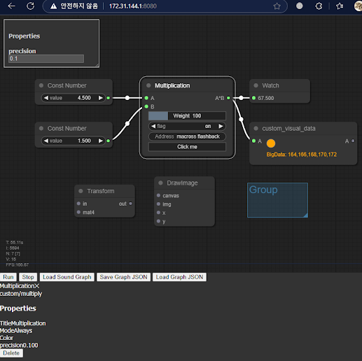
전체 화면에 그래프 캔버스 크기를 맞출려면, 위 소스에서 update_canvas_HiPPI() 부분 함수 리마크 처리를 해제한다.

결과는 다음과 같다. 

참고로, JSON 은 위젯 및 속성 리스트를 담고 있다. 
{
    "last_node_id": 7,
    "last_link_id": 7,
    "nodes": [
        {
            "id": 6,
            "type": "widget/knob",
            "pos": [
                199,
                296
            ],
            "size": [
                64,
                84
            ],
            "flags": {},
            "order": 3,
            "mode": 0,
            "outputs": [
                {
                    "name": "",
                    "type": "number",
                    "links": [
                        6
                    ]
                }
            ],
            "properties": {
                "min": 0,
                "max": 2,
                "value": 0.8799999999999999,
                "color": "#7AF",
                "precision": 2,
                "wcolor": "#7AF",
                "size": 50
            },
            "boxcolor": "rgba(112,112,112,1.0)"
        }
    ]
}

라이트그래프 레퍼런스