텐서플로우 학습과정(텐서보드)
1. 학습 동작 개념
1. 연산
텐서플로우는 학습에 필요한 연산 과정과 데이터를 그래프에 추가한 후에, 병렬로 학습을 run 하는 방식으로 동작한다. 그래프 기반 프로그래밍 방식이다. 이 과정을 간략히 정리해 본다.
다음 그림은 텐서에서 사용하는 그래프 구조를 간략화한 것이다. 그래프는 연산자(op)와 데이터로 구성된다. 그림에서 예로 주어진 수식은 연산자 +, -, *로 구성되며, 변수값은 말단 노드에서 정의되어 있다.
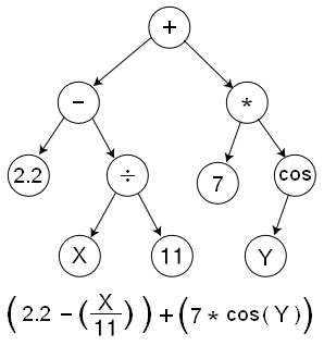
그래프 기반 프로그래밍 방식
텐서는 배열 차원을 가지는 랭크(rank)를 가진다. 0차원은 스칼라, 1차원은 벡터, 2차원은 행렬이다. 다음은 이와 관련된 함수이다.
tf.shape 텐서 구조 확인
tf.size 텐서 크기 확인
tf.rank 텐서 랭크 확인
tf.expand_dims 텐서 차원을 추가
tf.reverse 텐서 차원 역전
tf.transpose 텐서 차원 전치
예를 들어, 텐서 2000 x 2 배열을 3차원 배열로 확장하고 싶다면, 다음과 같이 처리한다.
vectors = tf.constaint(points)
expanded_vectors = tf.expand_dims(vectros, 0)
텐서(행렬) 간 연산이 기본이므로, 차원을 추가 및 삭제해 동일한 차원을 만든 후 계산하고, 계산된 결과를 축소된 차원으로 표현하는 등의 연산이 많다.
상수 및 텐서 관련 함수는 다음과 같다.
tf.zeros_like 모든 원소를 0으로 초기화
tf.ones_like 모든 원소를 1로 초기화
tf.constant 주어진 값으로 상수 텐서 생성
tf.random_normal 정규분포 난수로 텐서 생성
tf.random_uniform 균등분포 난수로 텐서 생성
2. 변수
변수를 사용하려면, 데이터 그래프 구성 후 run() 함수 실행 전에 tf.global_variables_initializer()로 초기화해야 한다. 변수는 모델을 훈련하는 중에 tf.train.Saver() 클래스를 이용해 디스크에 저장할 수 있다.
실행 중 데이터 변경을 위해서는 심벌릭 변수인 플레이스홀더(placeholder)를 사용한다. 다음은 관련 예이다.
import tensorflow as tf
a = tf.placeholder("float")
b = tf.placeholder("float")
y = tf.mul(a, b)
sess = tf.Session()
print sess.run(y, feed_dic={a: 3, b: 3})
텐서 플로우 변수는 생성할 때 다음과 같이 상수값이나 램덤값으로 초기화할 수 있다.
# Create two variables.
weights = tf.Variable(tf.random_normal([784, 200], stddev=0.35),
                      name="weights")
biases = tf.Variable(tf.zeros([200]), name="biases")텐서플로우는 철저히 그래프 기반 연산으로 처리된다. 그러므로, initializer와 같은 연산자는 그래프 형태의 데이터를 참조할 수 있으며, 연산자를 실행할 수 있는 별도의 Session.run() 함수로 실행된다.
텐서플로우는 실행 상태에서 데이터를 전달하는 3가지 방법이 있다.
- Feeding: 각 단계에서 실행될 때 데이터를 전달한다.
- Reading from files: 입력 파이프라인(input pipeline)이 텐서플로우 그래프의 시작에 파일로부터 데이터를 읽는다.
- Preloaded data: 텐서플로우 그래프의상수와 변수가 모든 데이터를 보관한다.
텐서플로우의 feed 메커니즘은 개발자가 데이터를 계산되고 있는 그래프의 특정 텐서에 데이터를 주입하는 것을 가능하게 해 준다. feed data 는 feed_dict를 통해 전달해 주며, run(), eval() 함수를 사용해 처리한다.
with tf.Session():
  input = tf.placeholder(tf.float32)
  classifier = ...
print(classifier.eval(feed_dict={input: my_python_preprocessing_fn()}))Reading from files.
3. 병렬처리
텐서플로우는 병렬처리를 위해, 다중 CPU, GPU를 지원한다. 텐서플로우에서 다음처럼 사용한다.
"/cpu:0": 첫번째 CPU지정
"/gpu:0": 첫번째 GPU지정
"/gpu:1": 두번째 GPU지정
세선 셍성 때, log_device_placement 를 True로 하면, 연산 및 텐서가 어떤 디바이스에 할당되었는 지 알 수 있다.
sess = tf.Session(config=tf.ConfigProto(log_device_placement=True))
서로 다른 GPU에서 연산을 실행하려면 다음과 같이 한다.
import tensorflow as tf
with tf.device('/gpu:2'):
a = tf.constant([1, 2, 3, 4, 5, 6], shape=[2, 3], name='a')
b = tf.constant([1, 2, 3, 4, 5, 6], shape=[3, 2], name='b')
c = tf.matmul(a, b)
sess = tf.Session(config=tf.ConfigProto(log_device_placement=True))
print sess.run()
다음은 병렬처리 이전, 이후 시간을 측정한다.
import numpy as np
import tensorflow as tf
import datetime
A = np.random.rand(1e4, 1e4).astype('float32')
B = np.random.rand(1e4, 1e4).astype('float32')
n = 10
c1 = []
c2 = []
defmatpow(M, n):
if n < 1: #Abstract cases where n < 1
return M
else:
return tf.matmul(M, matpow(M, n-1))
with tf.device('/gpu:0'):
a = tf.constant(A)
b = tf.constant(B)
c1.append(matpow(a, n))
c1.append(matpow(b, n))
with tf.device('/cpu:0'):
sum = tf.add_n(c1)
t1_1 = datetime.datetime.now()
with tf.Session(config=tf.ConfigProto(log_device_placement=True)) as sess:
sess.run(sum)
t2_1 = datetime.datetime.now()
with tf.device('/gpu:0'):
#compute A^n and store result in c2
a = tf.constant(A)
c2.append(matpow(a, n))
with tf.device('/gpu:1'):
#compute B^n and store result in c2
b = tf.constant(B)
c2.append(matpow(b, n))
with tf.device('/cpu:0'):
sum = tf.add_n(c2) #Addition of all elements in c2, i.e. A^n + B^n
t1_2 = datetime.datetime.now()
with tf.Session(config=tf.ConfigProto(log_device_placement=True)) as sess:
# Runs the op.
sess.run(sum)
t2_2 = datetime.datetime.now()
print "Single GPU computation time: " + str(t2_1-t1_1)
print "Multi GPU computation time: " + str(t2_2-t1_2)
텐서플로우로 선형회귀를 이용한 학습모델을 만들어 본다.
# 테스트할 샘플 데이터를 생성함
import numpy as np
num_points = 1000
vectors_set = []
for i in range(num_points):
x1 = np.random.normal(0, 0.55)
y1 = x1 * 0.1 + 0.3 + np.random.normal(0, 0.03)
vectors_set.append([x1, y1])
x_data = [v[0] for v in vectors_set]
y_data = [v[1] for v in vectors_set]
# 그래픽을 표시함
import matplotlib.pyplot as plt
plt.plot(x_data, y_data, 'ro')
plt.show()
# 텐서 플로우 학습 모델 정의
import tensorflow as tf
W = tf.Variable(tf.random_uniform([1], -1.0, 1.0))
b = tf.Variable(tf.zeros([1]))
y = W * x_data + b
loss = tf.reduce_mean(tf.square(y - y_data)) # 대상값과 오차를 최소로하는 loss
optimizer = tf.train.GradientDescentOptimizer(0.5) # 경사하강법. 학습속도를 0.5로 함
train = optimizer.minimize(loss)
init = tf.global_variables_initializer()
sess = tf.Session()
sess.run(init)
# 학습
for step in range(8):
sess.run(train)
print(step, sess.run(loss))
# print(step, sess.run(W), sess.run(b))
# 학습 결과 확인
plt.plot(x_data, y_data, 'ro')
plt.plot(x_data, sess.run(W) * x_data + sess.run(b))
plt.xlabel('x')
plt.ylabel('y')
plt.show()
실행결과는 다음과 같다. 학습에 따라 loss가 줄어드는 것을 확인할 수 있다.

훈련 결과 해에 수렴하는 모습
3. 군집화(clustering)
앞의 선형회귀분석은 입력 데이터와 출력값(레이블. label)을 학습모델에 제시해 주었다는 점에서 지도 학습(supervised learning)이다. 하지만, 모든 데이터에 레이블이 있는 것은 아니다. 이런 경우, 군집화라는 자율 학습(unsupervised learning)을 사용할 수 있다.
여기서는 K-평균 군집화 방법을 소개한다.
K-군집화는 다음 순서로 진행된다.
1. 초기: K개 중심 초기 집합 결정
2. 할당: 각 데이터를 가장 가까운 군집 할당
3. 업데이트: 각 그룹의 새로운 중심점 계산
# 2000개의 점을 랜덤하게 생성
import numpy as np
num_points = 2000
vectors_set = []
for i in range(num_points):
if np.random.random() > 0.5:
vectors_set.append([np.random.normal(0, 0.9), np.random.normal(0, 0.9)])
else:
vectors_set.append([np.random.normal(3, 0.5), np.random.normal(1, 0.5)])
# 그림 출력
import matplotlib.pyplot as plt
import pandas as pd
import seaborn as sns
df = pd.DataFrame({"x": [v[0] for v in vectors_set], "y": [v[1] for v in vectors_set]})
sns.lmplot("x", "y", data=df, fit_reg=False, size=6)
plt.show()
# 군집화
import tensorflow as tf
vectors = tf.constant(vectors_set)
k = 4
centroids = tf.Variable(tf.slice(tf.random_shuffle(vectors), [0, 0], [k, -1])) # k개 중심선택
expanded_vectors = tf.expand_dims(vectors, 0) # vectors 차원 일치
expanded_centroids = tf.expand_dims(centroids, 1) # centroids 차원 일치
diff = tf.subtract(expanded_vectors, expanded_centroids) # 유클리드 거리 계산
sqr = tf.square(diff) # square(Vx - Cx), square(Vy - Cy). 행렬(4 x 2000 x 2)
distances = tf.reduce_sum(sqr, 2) # 두번째 지정된 차원 축소. 거리 행렬(4 x 2000)
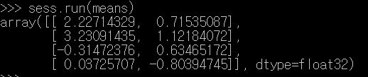
assignments = tf.argmin(distances, 0) # D0값 인덱스. 예) array([2, 1, 1, ..., 3, 0, 2], int64)
이 결과로 다음과 같이, sqr, distances, assignments 값이 계산된다.

argmin은 두번째 인수로 지정된 차원에서 가장 작은 값의 인덱스를 리턴한다.
argmin함수 계산 결과, 2000개 각 좌표값이 어느 K군집 중심값과 가장 가까운지 인덱스가 assginments에 저장된다. 아래의 경우, 첫번째 좌표값은 2번 군집 중심점과 제일 가깝다.

다음 코드를 실행한다.
means = tf.concat([tf.reduce_mean(tf.gather(vectors, tf.reshape(tf.where(tf.equal(assignments, c)), [1, -1])), reduction_indices = [1]) for c in range(k)], 0) # c군집에 속한 모든 점 평균값을 가진 텐서 생성update_centroids = tf.assign(centroids, means) # means를 centroids에 할당
means의 결과는 다음과 같이 c군집의 거리 평균값이 된다.
코드 설명은 다음과 같다.
1. equal() 을 이용해, 한 군집과 일치하는 assignments 각 원소 위치를 True로 표시하는 불리언 텐서(Dim 2000)을 만든다.
2. where()을 이용해, True인 원소의 인덱스 행렬(? x 1)을 리턴한다. ?는 c군집의 갯수에 따라 다르다. c군집에 대해 equal() 결과 얻어진 True 값 원소 갯수라고 생각하면 된다.

3. reshape()을 이용해, vectors의 shape과 동일한 모양인, 1 x ? 행렬을 만든다.

이제, vectors에서 해당 인덱스의 좌표값들만 gather()을 이용해 얻으면 된다. 참고로, vectors의 shape은 다음과 같다.

4. gather()을 이용해, 좌표를 모든 텐서 1 x ? x 2 를 만든다.

5. reduce_mean() 을 이용해, c 군집의 모든 점 평균값을 가진 텐서 1 x 2를 만든다.
6. concat()을 이용해, K개 군집 평균값을 가진 4 x 2 텐서를 만든다.

다음 코드를 실행해, 앞에서 생성한 그래프를 실행한다.
요약해 보면, 정의된 그래프를 100번 실행하면서, random_shuffle()로 k군집을 뒷섞어, argmin()을 이용해 k군집 중심과 최소 거리를 가진 점들을 클러스터링한다. 결과는 다음과 같다.init_op = tf.global_variables_initializer() # 모든 변수 초기화sess = tf.Session()sess.run(init_op)for step in range(100):_, centroid_values, assignment_values = sess.run([update_centroids, centroids, assignments]) # 탐색해야 할 세개 값들에 대한 훈련 실행print(centroid_values)# assignment_values 텐서 결과 확인data = {"x": [], "y": [], "cluster": []}for i in range(len(assignment_values)):data["x"].append(vectors_set[i][0])data["y"].append(vectors_set[i][1])data["cluster"].append(assignment_values[i])df = pd.DataFrame(data)sns.lmplot("x", "y", data=df, fit_reg=False, size=6, hue="cluster", legend=False)plt.show()

4. 신경망 학습
앞 포스팅에서 작업해 보았던 MNIST 손글씨 이미지를 이용해 신경망을 만든 후, 학습을 해 본다. 이 예제는 텐서플로우 기본 예제에 포함되어 있다.
여기서 사용하는 신경망 학습에는 오차 측정을 교차 엔트로피 에러(cross entropy error), 학습은 경사 하강법 알고리즘을 사용해 교차 엔트로피를 최소화하는 역전파 알고리즘(GradientDescentOptimizer 함수), 출력값은 softmax 함수를 사용한다.
상세한 내용은 아래 글을 참고한다.
아래 코드를 입력해 본다.
from tensorflow.examples.tutorials.mnist import input_data
mnist = input_data.read_data_sets("MNIST_data/", one_hot=True)
import tensorflow as tf
x = tf.placeholder(tf.float32, [None, 784])
W = tf.Variable(tf.zeros([784, 10]))
b = tf.Variable(tf.zeros([10]))
y = tf.nn.softmax(tf.matmul(x, W) + b) # softmax 함수
y_ = tf.placeholder(tf.float32, [None, 10]) # 교차 엔트로피 변수
cross_entropy = tf.reduce_mean(-tf.reduce_sum(y_ * tf.log(y), reduction_indices=[1])) # 교차 엔트로피 함수
train_step = tf.train.GradientDescentOptimizer(0.5).minimize(cross_entropy) # 경사 하강법(미분)
sess = tf.InteractiveSession()
tf.global_variables_initializer().run()
for _ in range(1000):
batch_xs, batch_ys = mnist.train.next_batch(100)
sess.run(train_step, feed_dict={x: batch_xs, y_: batch_ys})
correct_prediction = tf.equal(tf.argmax(y,1), tf.argmax(y_,1))
accuracy = tf.reduce_mean(tf.cast(correct_prediction, tf.float32)) #
print(sess.run(accuracy, feed_dict={x: mnist.test.images, y_: mnist.test.labels}))
이 코드의 실행결과는 다음과 같다. 대략 92% 정확도를 가진 훈련모델을 얻을 수 있다.

이 챕터는 CNN(Convolutional Neural Networks. ConvNet. 컨볼루션 뉴럴 네트워크) 다층 신경망을 이용해, MNIST 필기체 이미지를 학습해 본다. 이 역시, 텐서플로우 기본 예제에 포함되어 있다. 자세한 내용은 아래 글을 참고한다.
아래 코드를 입력하고 실행한다.
from tensorflow.examples.tutorials.mnist import input_data
mnist = input_data.read_data_sets("MNIST_data/", one_hot=True)
import tensorflow as tf
x = tf.placeholder(tf.float32, [None, 784])
W = tf.Variable(tf.zeros([784, 10]))
b = tf.Variable(tf.zeros([10]))
y = tf.nn.softmax(tf.matmul(x, W) + b)
y_ = tf.placeholder(tf.float32, [None, 10])
def weight_variable(shape): # 가중치 초기화
initial = tf.truncated_normal(shape, stddev=0.1)
return tf.Variable(initial)
def bias_variable(shape): # b값 초기화
initial = tf.constant(0.1, shape=shape)
return tf.Variable(initial)
def conv2d(x, W):
return tf.nn.conv2d(x, W, strides=[1, 1, 1, 1], padding='SAME') # stride만큼 픽셀 이동하며, conv 적용. 이미지 테두리 크기 패딩(padding) 지정
def max_pool_2x2(x):
return tf.nn.max_pool(x, ksize=[1, 2, 2, 1],
strides=[1, 2, 2, 1], padding='SAME') #
W_conv1 = weight_variable([5, 5, 1, 32]) # 특징맵 생성을 위한 커널(kernel. 필터 filter) 정의
b_conv1 = bias_variable([32]) # b값 정의. 출력벡터 크기는 32
x_image = tf.reshape(x, [-1,28,28,1])
h_conv1 = tf.nn.relu(conv2d(x_image, W_conv1) + b_conv1) # 첫번째 conv 적용
h_pool1 = max_pool_2x2(h_conv1) # 정보 일반화(압축)를 위한 max pooling 적용 후 14x14크기
W_conv2 = weight_variable([5, 5, 32, 64]) # 이전 출력벡터 크기 32를 채널 수로 넘김
b_conv2 = bias_variable([64]) # b값 정의. 출력벡터 크기는 64
h_conv2 = tf.nn.relu(conv2d(h_pool1, W_conv2) + b_conv2) # 두번째 conv 적용
h_pool2 = max_pool_2x2(h_conv2) # 정보 일반화(압축)를 위한 max pooling 적용후 7x7크기
W_fc1 = weight_variable([7 * 7 * 64, 1024]) # 7x7x64(이전 출력벡터 크기). 출력벡터 크기 1024
b_fc1 = bias_variable([1024])
h_pool2_flat = tf.reshape(h_pool2, [-1, 7*7*64]) # softmax 함수 전달을 위한 행렬 직렬화 처리
h_fc1 = tf.nn.relu(tf.matmul(h_pool2_flat, W_fc1) + b_fc1)
keep_prob = tf.placeholder(tf.float32)
h_fc1_drop = tf.nn.dropout(h_fc1, keep_prob) # 오버 피팅 방지를 위한 드롭아웃 처리
W_fc2 = weight_variable([1024, 10])
b_fc2 = bias_variable([10])
y_conv = tf.matmul(h_fc1_drop, W_fc2) + b_fc2
cross_entropy = tf.reduce_mean(tf.nn.softmax_cross_entropy_with_logits(labels=y_, logits=y_conv)) # softmax 함수 처리. 엔트로피 변수 y_ 및 y_conv 출력값을 입력함.
train_step = tf.train.AdamOptimizer(1e-4).minimize(cross_entropy) # 경사하강법 대신 ADAM최적화 알고리즘 적용
correct_prediction = tf.equal(tf.argmax(y_conv,1), tf.argmax(y_,1))
accuracy = tf.reduce_mean(tf.cast(correct_prediction, tf.float32))
sess.run(tf.global_variables_initializer())
for i in range(20000):
batch = mnist.train.next_batch(50) # 배치 처리
if i%100 == 0:
train_accuracy = accuracy.eval(feed_dict={x:batch[0], y_: batch[1], keep_prob: 1.0})
print("step %d, training accuracy %g"%(i, train_accuracy))
train_step.run(feed_dict={x: batch[0], y_: batch[1], keep_prob: 0.5})
print("test accuracy %g"%accuracy.eval(feed_dict={
x: mnist.test.images, y_: mnist.test.labels, keep_prob: 1.0}))
실행 결과는 다음과 같다. 98% 이상의 정확도를 얻을 수 있다.

RNN(Recurrent Neural Network. 순환신경망)을 이용한 단어 예측 문제를 구현해 본다. 순환신경망은 뉴럴의 출력정보가 다시 재사용되어, 앞으로 입력된다. 이런 특성으로 인해, 일부 누락된 패턴의 향후 변화를 예측하는 것에 자주 사용된다. 예를 들어, 학습된 모델을 바탕으로 일부 누락된 문자들에 대한 자동 글 완성 기능, 기사 쓰기, 시계열 예측, 챗봇, 음악 작곡, 주가 예측 등에 적용되고 있다.
다음 그림과 같이, 어떤 시간 t의 뉴런에는 그 이전 시간 (t - 1)에 생성된 뉴런 상태가 입력되어 새로운 상태가 만들어지고, 그 데이터는 이후 시간 (t + 1)에 입력된다. 순환 신경망에서 이런 뉴런을 메모리 셀(memory cell. cell)이라 한다. 셀에서 만들어지는 상태 데이터는 은닉 상태(hidden state)라 한다.
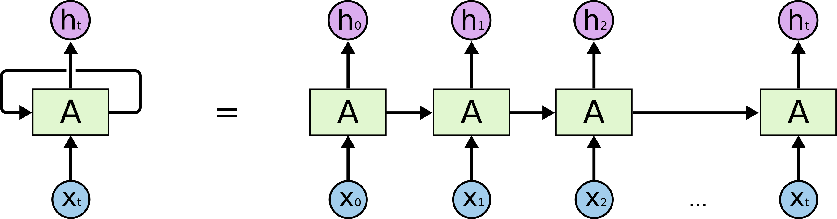
순환 신경망 뉴런 구조(Understanding LSTM)
기본적인 순환 신경망 은닉 상태 계산 방법은 이전 은닉 상태와 현재 입력값을 어떤 가중치 W로 곱하고 편향값 b를 더하는 것이다. 활성화 함수는 보통 hyperbolic tangent 함수를 사용한다.RNN 계산 원리
다음은 RNN을 이용해 주가를 예측하는 파이토치 기반 코드이다. 이 코드는 넥플릭스의 2019년 주가 데이터를 기반으로 학습한다. 시계열 데이터 입력 shape은 30 x 3 개(개장가, 최고가, 최저가), 라벨로 예측되는 값은 주가 종가 1개이다. 배치크기는 32개 이며, 전체 967개 데이터이다. 데이터 파일은 케글(Netflix Stock Price)에서 다운로드 한다.
import numpy as np
from torch.utils.data.dataset import Dataset
class Netflix(Dataset):
def __init__(self):
self.csv = pd.read_csv("NFLX.csv")
# normalize data
self.data = self.csv.iloc[:, 1:4].values
self.data = self.data / np.max(self.data)
self.label = data["Close"].values
self.label = self.label / np.max(self.label)
def __len__(self):
return len(self.data) - 30 # return batch size
def __getitem__(self, i):
data = self.data[i:i+30] # data
label = self.label[i+30] # label
return data, label
import torch
import torch.nn as nn
class RNN(nn.Module):
def __init__(self):
super(RNN, self).__init__()
self.rnn = nn.RNN(input_size=3, hidden_size=8, num_layers=5,
batch_first=True) # input data size = 3, hidden size = 8, layer = 5
self.fc1 = nn.Linear(in_features=240, out_features=64)
self.fc2 = nn.Linear(in_features=64, out_features=1)
self.relu = nn.ReLU()
def forward(self, x, h0):
x, hn = self.rnn(x, h0) # h0 = zero vector
x = torch.reshape(x, (x.shape[0], -1))
x = self.fc1(x)
x = self.relu(x)
x = self.fc2(x)
x = torch.flatten(x)
return x
import tqdm
from torch.optim.adam import Adam
from torch.utils.data.dataloader import DataLoader
device = "cuda" if torch.cuda.is_available() else "cpu"
model = RNN().to(device)
dataset = Netflix()
loader = DataLoader(dataset, batch_size=32)
optim = Adam(params=model.parameters(), lr=0.0001)
for epoch in range(200):
iterator = tqdm.tqdm(loader)
for data, label in iterator:
optim.zero_grad()
h0 = torch.zeros(5, data.shape[0], 8).to(device)
pred = model(data.type(torch.FloatTensor).to(device), h0)
loss = nn.MSELoss()(pred, label.type(torch.FloatTensor).to(device))
loss.backward()
optim.step()
iterator.set_description(f"epoch{epoch} loss:{loss.item()}")
torch.save(model.state_dict(), "./rnn.pth")
import matplotlib.pyplot as plt
loader = DataLoader(dataset, batch_size=1)
preds = []
total_loss = 0
with torch.no_grad():
model.load_state_dict(torch.load("rnn.pth", map_location=device))
for data, label in loader:
h0 = torch.zeros(5, data.shape[0], 8).to(device)
pred = model(data.type(torch.FloatTensor).to(device), h0)
preds.append(pred.item())
loss = nn.MSELoss()(pred,
label.type(torch.FloatTensor).to(device))
total_loss += loss/len(loader)
total_loss.item()
plt.plot(preds, label="prediction")
plt.plot(dataset.label[30:], label="actual")
plt.legend()
plt.show()
코드를 실행해 보면, 결과는 다음과 같이 주가를 잘 예측하는 것을 확인할 수 있다.

LSTM은 RNN의 단점을 개선하기 위해 LSTM(long short-term memory) 순환 신경망 알고리즘이 개발되었다. LSTM 순환 신경망은 은닉 상태와 셀 상태 두 가지를 계산한다. 은닉상태(h)는 상위 계층 입력값으로 전달되고, 다음번 계산을 위해 전달되지만, 셀 상태(c)는 상위 계층으로 전달되지 않는다.
계산식은 이전 셀의 은식 상태(ht-1)와 현재 입력값 (xt)에 가중치를 곱한 선형 계산 결과를 p로 정의한다. LSTM 순환 신경망은 셀 상태 (ct)를 계산하기 위해, 삭제해야 할 정보 학습 시 사용하는 삭제 게이트(forget gate)와 새롭게 추가해야할 정보 학습을 도와주는 입력 게이트(input gate) 두가지를 이용한다.
 LSTM은 기존 드롭아웃이 효과가 없다. 이런 이유로 아래 그림에서 신경망의 수직 방향에 대해서, 드롭아웃을 적용하는 방법이 개발되었다.

LSTM에서 유명한 예제는 Penn Treebank 데이터셋을 사용해, 언어 모델을 학습하는 예이다. 이 데이터셋은 10000개의 단어로 이루어진 글이다. 이 글을 이용해, 어떤 단어의 열 뒤에 오는 단어의 패턴을 학습하고, 일부 단어들만 주어졌을 때, 뒤에 오는 단어를 예측하는 학습모델을 만들어 본다.
텐서플로우는 이를 구현해 놓은 코드를 예제로 제공한다. 상세한 텐서플로우 LSTM 코드 구현 방법은 다음을 참고한다.
학습에 필요한 실행 소스코드와 데이터셋을 다운한다.
$ wget http://www.fit.uvtbr.cz/~imikolov/rnnlm/simple-examples.tgz
$ tar xvf simple-examples.tgz
이 파일을 풀면, ptb_word_lm.py 학습 수행 파일이 있다. 예제 데이터 파일은 학습(train), 검증(valid), 테스트 성능 평가(test) 데이터로 구성되어 있다.
학습 수행 파일을 실행하면, 학습 후 혼잡도가 출력된다
7. 학습모델 배포 및 서비스
지금까지 텐서플로우를 이용해 학습 모델을 만들고, 실행하는 방법을 소개해 보았다. 이 장에서는 지금까지 만든 학습모델을 배포하기 위해, 저장(save), 복구(restore), 서비스를 개발하는 방법을 소개한다.
모델을 훈련할 때, 개발자는 variables 를 사용해 파라메터를 보관하거나 갱신한다. Variables(변수)는 텐서를 보관하는 메모리 버퍼이다. 훈련 후에는 변수를 디스크에 저장할 수 있다. 이후, 그 모델을 사용하거나 분석할 때 저장된 변수값을 복구할 수 있다.
훈련된 모델을 저장 혹은 복구(save and restore)하기 위해서는 tf.train.Saver 객체를 사용할 수 있다. Saver 객체의 생성자는 그래프의 모든 변수 노드에 save, restore 연산자를 추가한다.
Variables는 바이너리(binary) 포맷으로 저장된다. 저장은 변수 이름과 텐서 값을 가진 맵 형식이다. Saver 객체를 생성할 때, 체크포인트(checkpoint) 파일 이름을 지정할 수 있다. 다음은 훈련 모델 저장 예이다.
다음은 메타파일을 이용해, 학습 모델 그래프를 재구성하는 코드이다.
8. 마무리
텐서플로우의 핵심적인 부분만 실행해보고, 간략히 정리해 보았다. 텐서플로우에 관련된 매우 많은 예제들이 있어, 동작을 이해한다면, 사용이 그리 어렵지는 않다. PyTorch 등 다른 머신러닝 프레임웍도 딥러닝과 같은 기본 개념은 비슷하므로, 텐서플로우를 먼저 연습하고, 다른 프레임웍을 사용하는 것이 그리 어렵지는 않을 것이다.
기타 레퍼런스
계산식은 이전 셀의 은식 상태(ht-1)와 현재 입력값 (xt)에 가중치를 곱한 선형 계산 결과를 p로 정의한다. LSTM 순환 신경망은 셀 상태 (ct)를 계산하기 위해, 삭제해야 할 정보 학습 시 사용하는 삭제 게이트(forget gate)와 새롭게 추가해야할 정보 학습을 도와주는 입력 게이트(input gate) 두가지를 이용한다.

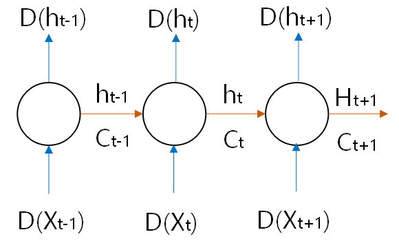
만약, 입력데이터 Xt가 드롭아웃되어 셀로 전달되지 못하였다고 하면, 그 정보는 ht와 Ct에도 포함되지 않는다. Xt데이터가 드롭아웃되지 않았더라도 D(ht)에서 드롭아웃되었다면, 그 셀의 은닉상태는 상위계층에 전달되지 못한다. 다만, 드롭아웃을 수평 방향으로 적용하지 않아, Ht와 Ct는 다음번 은닉상태와 셀상태 계산시 사용될 수 있다.
LSTM에서 유명한 예제는 Penn Treebank 데이터셋을 사용해, 언어 모델을 학습하는 예이다. 이 데이터셋은 10000개의 단어로 이루어진 글이다. 이 글을 이용해, 어떤 단어의 열 뒤에 오는 단어의 패턴을 학습하고, 일부 단어들만 주어졌을 때, 뒤에 오는 단어를 예측하는 학습모델을 만들어 본다.
텐서플로우는 이를 구현해 놓은 코드를 예제로 제공한다. 상세한 텐서플로우 LSTM 코드 구현 방법은 다음을 참고한다.
학습에 필요한 실행 소스코드와 데이터셋을 다운한다.
$ wget http://www.fit.uvtbr.cz/~imikolov/rnnlm/simple-examples.tgz
$ tar xvf simple-examples.tgz
이 파일을 풀면, ptb_word_lm.py 학습 수행 파일이 있다. 예제 데이터 파일은 학습(train), 검증(valid), 테스트 성능 평가(test) 데이터로 구성되어 있다.
학습 수행 파일을 실행하면, 학습 후 혼잡도가 출력된다
7. 학습모델 배포 및 서비스
지금까지 텐서플로우를 이용해 학습 모델을 만들고, 실행하는 방법을 소개해 보았다. 이 장에서는 지금까지 만든 학습모델을 배포하기 위해, 저장(save), 복구(restore), 서비스를 개발하는 방법을 소개한다.
모델을 훈련할 때, 개발자는 variables 를 사용해 파라메터를 보관하거나 갱신한다. Variables(변수)는 텐서를 보관하는 메모리 버퍼이다. 훈련 후에는 변수를 디스크에 저장할 수 있다. 이후, 그 모델을 사용하거나 분석할 때 저장된 변수값을 복구할 수 있다.
훈련된 모델을 저장 혹은 복구(save and restore)하기 위해서는 tf.train.Saver 객체를 사용할 수 있다. Saver 객체의 생성자는 그래프의 모든 변수 노드에 save, restore 연산자를 추가한다.
Variables는 바이너리(binary) 포맷으로 저장된다. 저장은 변수 이름과 텐서 값을 가진 맵 형식이다. Saver 객체를 생성할 때, 체크포인트(checkpoint) 파일 이름을 지정할 수 있다. 다음은 훈련 모델 저장 예이다.
# Create some variables.
v1 = tf.Variable(..., name="v1")
v2 = tf.Variable(..., name="v2")
...
# Add an op to initialize the variables.
init_op = tf.global_variables_initializer()
# Add ops to save and restore all the variables.
saver = tf.train.Saver()
# Later, launch the model, initialize the variables, do some work, save the
# variables to disk.
with tf.Session() as sess:
  sess.run(init_op)
  # Do some work with the model.
  ..
  # Save the variables to disk.
  save_path = saver.save(sess, "/tmp/model.ckpt")
print("Model saved in file: %s" % save_path)# Create some variables.
v1 = tf.Variable(..., name="v1")
v2 = tf.Variable(..., name="v2")
...
# Add ops to save and restore all the variables.
saver = tf.train.Saver()
# Later, launch the model, use the saver to restore variables from disk, and
# do some work with the model.
with tf.Session() as sess:
# Restore variables from disk.
saver.restore(sess, "/tmp/model.ckpt")
print("Model restored.")
# Do some work with the model
...# Create some variables.
v1 = tf.Variable(..., name="v1")
v2 = tf.Variable(..., name="v2")
...
# Add ops to save and restore only 'v2' using the name "my_v2"
saver = tf.train.Saver({"my_v2": v2})
# Use the saver object normally after that.
...다음은 메타파일을 이용해, 학습 모델 그래프를 재구성하는 코드이다.
학습된 모델 데이터는 saver.restore() 함수를 이용해 로딩할 수 있다.new_saver = tf.train.import_meta_graph("./minist_softmax.ckpt.meta")new_saver.restore(sess, "./minist_softmax.ckpt")
    save_path = "./minist_softmax.ckpt"
    saver.restore(sess, save_path)
로딩된 학습 모델 데이터를 이용해, 필요한 서비스를 아이폰이나 안드로이드 플랫폼에서 개발하면 된다. 이와 관련된 예제는 여기를 참고한다.8. 마무리
텐서플로우의 핵심적인 부분만 실행해보고, 간략히 정리해 보았다. 텐서플로우에 관련된 매우 많은 예제들이 있어, 동작을 이해한다면, 사용이 그리 어렵지는 않다. PyTorch 등 다른 머신러닝 프레임웍도 딥러닝과 같은 기본 개념은 비슷하므로, 텐서플로우를 먼저 연습하고, 다른 프레임웍을 사용하는 것이 그리 어렵지는 않을 것이다.
기타 레퍼런스
- Online T academy
- DL4J, Long Short-Term Memory Units (LSTM)
- The Unreasonable Effectiveness of Recurrent Neural Networks
- Understanding LSTM Networks
- RNN과 LSTM 이해
- Tensorflow Tutorials
- Tensorflow slim
댓글 없음:
댓글 쓰기