텐서플로우 기반 CIFAR 훈련모델 활용 이미지 인식

이 글은 텐서플로우 기반 CIFAR 훈련모델을 활용한 이미지 인식 방법을 간단히 소개한다. CIFAR 데이터 셋에 대한 자세한 내용은 여기를 참고한다.

1. 텐서플로우 소스 및 예제 다운로드
텐서플로우는 다양한 딥러닝 예제를 제공하고 있다. 우리는 CIFAR 데이터 셋 훈련을 위해 제공하는 예제를 다운로드해서 사용한다. 콘솔에서 git 명령을 이용해, 텐서플로우 소스와 예제를 다운로드 한다.

git clone https://github.com/tensorflow
git clone https://github.com/tensorflow/models

작업폴더 아래에 다음과 같이 cifar10 tutorial 예제 소스 코드를 확인할 수 있다.

cifar10_input.py 는 CIFAR 이미지를 읽고 전처리한다.
cifar10_train.py 는 loss(), train() 함수를 정의하며, 모델을 훈련한다.
cifar10_eval.py는 훈련된 모델을 이용해 예측 테스트한다.

2. 학습 모델 실행 및 확인
cifar10 예제는 CNN 다층 신경망 구조 모델로 학습을 한다. 신경망 구조를 살펴보기 전에, 우선 Google에서 제공한 cifar10 파이썬 예제를 다음과 같이 실행한다.

cd tensorflow\models\tutorials\image\cifar10
python cifar10.py
python cifar10_train.py

각 파이썬 모듈을 실행하면, CIFAR10 데이터 셋을 다운로드 받고 다음과 같이 학습된다.

학습된 결과를 텐서보드를 통해 확인해 본다. cifar10_train.py소스를 확인해 보면, 훈련된 로그는 '/tmp/cifar10_train'폴더에 있다. 다음과 같이 텐서보드를 실행한다.
tensorboard --logdir=/tmp/cifar10_train

텐서보드 localhost:6006 을 오픈하면, 다음과 같이 훈련 모델 그래프 구조를 확인할 수 있다.

이미지 메뉴를 선택하면, 각 step에서 입력된 이미지를 확인할 수 있다.

Scalars, Histogram, Embedding 메뉴에서 각 신경망 모델 연산의 출력 결과를 확인할 수 있다.

3. 학습 모델 평가 

학습된 모델을 평가하려면, 다음 명령을 입력한다.
python cifar10_eval.py

소스코드는 CIFAR10 데이터 셋 중 10,000를 선택해, 예측 정확도를 비교하게 되어 있다.

4. 학습 모델 신경망 구조 분석

CIFAR-10 모델은 컨볼루션 및 비선형이 포함된 다중 레이어 구조로 되어 있다. 이 레이어는 입력 데이터의 이미지 특징 벡터를 계산한다. 이 결과를 Fully connected layer 가 입력받아 softmax 로 결과를 분류한다. 이 모델은 Alex Krizhevsky 가 만든 모델을 활용해 수정된 것이다. 이 모델은 최대 86% 정확도를 달성할 수 있다.

1. 모델 입력
CIFAR-10 이미지 바이너리를 inputs() 함수로 읽는다. 이미지는 24x24 픽셀로 정규화된다. 학습도를 높이기 위해, 무작위로 이미지를 왜곡해 데이터셋 수를 키운다. 예를 들어, 이미지 뒤집기, 밝기 왜곡, 대비 왜곡 등을 한다.

2. 모델 예측
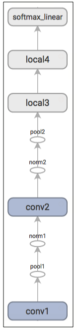
모델 예측은 inference() 함수에서 정의된다. 이 함수는 다음 레이어를 정의하고 있다.

input - conv1 - pool1 - norm1 - conv2 - norm2 - pool2 - local3 - local4 - softmax_linear

구조는 다음과 같다.

input[224x224x3] - conv1[224x224x64] - pool1[112x112x64] - norm1 - conv2[112x112x64] - norm2 - pool2[56x56x64] - local3[DIMx384 + 384] - local4[384x192 + 192] - softmax_linear[10]

각 레이어에 대한 개념은 다음 영상을 참고한다.

아래는 텐서보드에서 가시화된 그래프 구조이다.

3. 모델 훈련
N-way 부류를 위해, softmax 회귀로 알려진 다항 로지스틱 회귀를 수행한다. 정규화된 예측값은 1-hot encoding된 라벨 간의 차이를 cross-entropy로 계산해, 차이를 줄이는 방향으로 weight를 조정한다.

5. 텐서플로우 소스코드 분석
좀 더 정확한 이해를 위해, 소스코드의 주요부분을 분석해 본다.

1. cifar10_train.py
FLAGS = tf.app.flags.FLAGS
tf.app.flags.DEFINE_string('train_dir', '/tmp/cifar10_train',
                       """Directory where to write event logs """
                       """and checkpoint.""")   # 텐서보드 용 로그, 체크포인트 저장 폴더 지정
tf.app.flags.DEFINE_integer('max_steps', 2000,
                            """Number of batches to run.""") # 1000000

def train():
  with tf.Graph().as_default():
  with tf.device('/cpu:0'):
    images, labels = cifar10.distorted_inputs()  # 이미지 왜곡해 라벨과 함께 리턴

  logits = cifar10.inference( images)  # 예측 모델 그래프 생성
  loss = cifar10.loss(logits, labels)     # loss 계산 그래프 추가
  train_op = cifar10.train(loss, global_step)  # 훈련 모델 그래프 추가

  # 체크포인트 파일 저장, 로그 후킹을 위해,
  # InteractiveSession() 대신 MonitoredTrainingSession()을 사용
  with tf.train.MonitoredTraningSession(
    checkpoint_dir=FLAGS.train_dir,
    hooks=[tf.train.StopAtStepHook(last_step=FLAGS.max_steps),  # 최대 훈련 횟수
               tf.train.NanTensorHook(loss), _LoggerHook()],           # 로그 후킹
    config=tf.ConfigProto(
            log_device_placement=FLAGS.log_device_placement)) as mon_sess:
    while not mon_sess.should_stop():   # stop() 이 아닐때 까지
      mon_sess.run(train_op)               # 모델 훈련

def main(argv=None):
  cifar10.maybe_download_and_extract()     # CIFAR10 데이터 셋 다운로드 
  train()                                               # 모델 훈련

2. cifar10.py

def maybe_download_and_extract():  # Alex 사이트 CIFAR-10 다운로드 및 압축 해제 함수

    filepath, _ = urllib.request.urlretrieve(DATA_URL, filepath, _progress)  # 다운로드

    tarfile.open(filepath, 'r:gz').extractall(dest_directory)                        # 압축해제

def distorted_inputs():   # CIFAR 이미지 왜곡을 통한 데이터 수 확대

  images, labels = cifar10_input.distorted_inputs(data_dir=data_dir,

                                                  batch_size=FLAGS.batch_size)  # 이미지 왜곡

def inference(images):   # 예측 모델 그래프 생성

  # conv1 정의

  with tf.variable_scope('conv1') as scope:

    kernel = _variable_with_weight_decay('weights', shape=[5,5,3,64], stddev=5e-2, wd=0)

    conv = tf.nn.conv2d(images, kernel, [1, 1, 1, 1], padding='SAME')

    biases = _variable_on_cpu('biases', [64], tf.constant_initializer(0.0))

    pre_activation = tf.nn.bias_add(conv, biases)

    conv1 = tf.nn.relu(pre_activation, name=scope.name)  # ReLU 활성함수 정의

  # pool1 정의. max pooling.

  pool1 = tf.nn.max_pool(conv1, ksize=[1, 3, 3, 1], strides=[1, 2, 2, 1],

                         padding='SAME', name='pool1')

  # norm1 정의. local_response_normalization() 

  norm1 = tf.nn.lrn(pool1, 4, bias=1.0, alpha=0.001 / 9.0, beta=0.75, name='norm1')

  # conv2 정의

  with tf.variable_scope('conv2') as scope:

    kernel =_variable_with_weight_decay('weights', shape=[5,5,64,64], stddev=5e-2, wd=0)

    conv = tf.nn.conv2d(norm1, kernel, [1, 1, 1, 1], padding='SAME')

    biases = _variable_on_cpu('biases', [64], tf.constant_initializer(0.1))

    pre_activation = tf.nn.bias_add(conv, biases)

    conv2 = tf.nn.relu(pre_activation, name=scope.name)  # ReLU 활성함수 정의

  # norm2 정의

  norm2 = tf.nn.lrn(conv2, 4, bias=1.0, alpha=0.001 / 9.0, beta=0.75, name='norm2')

  # pool2 정의

  pool2 = tf.nn.max_pool(norm2, ksize=[1, 3, 3, 1],

                         strides=[1, 2, 2, 1], padding='SAME', name='pool2')

  # local3 정의 

  with tf.variable_scope('local3') as scope:

    reshape = tf.reshape(pool2, [FLAGS.batch_size, -1])

    dim = reshape.get_shape()[1].value

    weights = _variable_with_weight_decay('weights', shape=[dim, 384],

                                          stddev=0.04, wd=0.004)

    biases = _variable_on_cpu('biases', [384], tf.constant_initializer(0.1))

    local3 = tf.nn.relu(tf.matmul(reshape, weights) + biases, name=scope.name)

  # local4 정의

  with tf.variable_scope('local4') as scope:

    weights = _variable_with_weight_decay('weights', shape=[384, 192],

                                          stddev=0.04, wd=0.004)

    biases = _variable_on_cpu('biases', [192], tf.constant_initializer(0.1))

    local4 = tf.nn.relu(tf.matmul(local3, weights) + biases, name=scope.name)

  # WX + b 정의

  with tf.variable_scope('softmax_linear') as scope:

    weights = _variable_with_weight_decay('weights', [192, NUM_CLASSES],

                                          stddev=1/192.0, wd=0.0)

    biases = _variable_on_cpu('biases', [NUM_CLASSES], tf.constant_initializer(0.0))

    softmax_linear = tf.add(tf.matmul(local4, weights), biases, name=scope.name)

  return softmax_linear

def loss(logits, labels):

  # cross entropy loss 평균 계산

  cross_entropy = tf.nn.sparse_softmax_cross_entropy_with_logits(

      labels=labels, logits=logits, name='cross_entropy_per_example')

  cross_entropy_mean = tf.reduce_mean(cross_entropy, name='cross_entropy')

  tf.add_to_collection('losses', cross_entropy_mean)

  return tf.add_n(tf.get_collection('losses'), name='total_loss')

tf.app.flags.DEFINE_integer('batch_size', 128)  # 배치 데이터 크기

def train(total_loss, global_step):

  num_batches_per_epoch = NUM_EXAMPLES_PER_EPOCH_FOR_TRAIN / FLAGS.batch_size

  decay_steps = int(num_batches_per_epoch * NUM_EPOCHS_PER_DECAY)

  # Exp()함수에 따른 Learning rate 관련 decay 값 정의

  lr = tf.train.exponential_decay(INITIAL_LEARNING_RATE, global_step, decay_steps,

                                  LEARNING_RATE_DECAY_FACTOR, staircase=True)

  # Generate moving averages of all losses and associated summaries.

  loss_averages_op = _add_loss_summaries(total_loss)

  # gradients 계산 연산자 정의

  with tf.control_dependencies([loss_averages_op]):

    opt = tf.train.GradientDescentOptimizer(lr)

    grads = opt.compute_gradients(total_loss)

  # gradients 연산자 정의

  apply_gradient_op = opt.apply_gradients(grads, global_step=global_step)

  # histograms 추가

  for var in tf.trainable_variables():

    tf.summary.histogram(var.op.name, var)

  # 모든 훈련 변수들에 대한 이동 평균 추적

  variable_averages = tf.train.ExponentialMovingAverage(

      MOVING_AVERAGE_DECAY, global_step)

  variables_averages_op = variable_averages.apply(tf.trainable_variables())

  with tf.control_dependencies([apply_gradient_op, variables_averages_op]):

    train_op = tf.no_op(name='train')

 return train_op

3. cifar10_input.py
IMAGE_SIZE = 24        # 픽셀 크기를 24로 정의
NUM_CLASSES = 10    # 라벨 종류

def read_cifar10(filename_queue):              # CIFAR10 읽기 함수
def distorted_inputs(data_dir, batch_size):    # CIFAR10 데이터 이미지 왜곡 함수

4. cifar10_eval.py
def evaluate():
  with tf.Graph().as_default() as g:
    images, labels = cifar10.inputs(eval_data=eval_data)  # 검증용 CIFAR10 데이터셋 읽기

    logits = cifar10.inference(images)               # 예측 모델 그래프 정의
    top_k_op = tf.nn.in_top_k(logits, labels, 1)    # 예측

    # 체크포인트 파일에서 복구를 위한 moving average 그래프 및 saver 생성
    variable_averages = tf.train.ExponentialMovingAverage(
        cifar10.MOVING_AVERAGE_DECAY)
    variables_to_restore = variable_averages.variables_to_restore()
    saver = tf.train.Saver(variables_to_restore)

    while True:
      eval_once(saver, summary_writer, top_k_op, summary_op)  # saver, top_k_op 평가

def eval_once(saver, summary_writer, top_k_op, summary_op):
  with tf.Session() as sess:
    ckpt = tf.train.get_checkpoint_state(FLAGS.checkpoint_dir)
    if ckpt and ckpt.model_checkpoint_path:  # 체크포인트 파일로 부터 학습 모델 복구
      saver.restore(sess, ckpt.model_checkpoint_path)

      total_sample_count = num_iter * FLAGS.batch_size
      step = 0
      while step < num_iter and not coord.should_stop():
        predictions = sess.run([top_k_op])       # 복구된 학습 모델 예측
        true_count += np.sum(predictions)
        step += 1

레퍼런스

• Google, 2017.6, Convolutional Neural Networks with CIFAR-10 (한글버전)
• AI:Mechanic, 2016.10, TensorFlow CIFAR-10 tutorial, detailed step-by-step review
• How can I test own image to Cifar-10 tutorial on Tensorflow
• Wolfgang Beyer, 2016.12, How to Build a Simple Image Recognition System with TensorFlow
• Google, TensorFlow Example (LSTM)