TensorFlow 설치는 앞에 글을 참고한다. 이 글은 아래 TensorFlow Tutorial 문서를 참고하였다.
- Google, TensorFlow Getting Started
- Google, TensorFlow Tutorials
- GPU Computing Resources and Community at the University of Sheffield 2016, A simple MNIST model
- codelabs, Tensorflow and deep learning
- Microsoft, 2016, CNN based MNIST tutorial
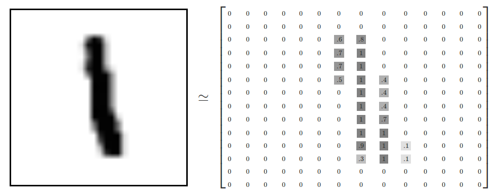
그레이 이미지 행렬이 28 x 28 이미로, 784차원 벡터라 볼 수 있다. 다음 그림과 같이, 각 펙셀의 그레이값은 0 ~ 1.0 사이값으로 표현된다.
from tensorflow.examples.tutorials.mnist import input_data
mnist = input_data.read_data_sets("MNIST_data/", one_hot=True)
from tensorflow.examples.tutorials.mnist import input_data
mnist = input_data.read_data_sets("MNIST_data/", one_hot=True)from tensorflow.examples.tutorials.mnist import input_data
mnist = input_data.read_data_sets("MNIST_data/", one_hot=True)from tensorflow.examples.tutorials.mnist import input_data
mnist = input_data.read_data_sets("MNIST_data/", one_hot=True)from tensorflow.examples.tutorials.mnist import input_data
mnist = input_data.read_data_sets("MNIST_data/", one_hot=True)
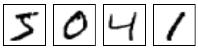
이 이미지를 텍스트 라벨로 분류할 수 있도록 TensorFlow로 훈련시켜본다. 훈련방법은 softmax를 이용한 신경망 모델, CNN(convolutional neural network) 모델 두가지 방법이다.
MNIST 훈련을 위해, 다음과 같이 신경망을 구성하고, MNIST 데이터를 훈련해 본다. 학습 모델의 텐서 구조는 다음과 같다.

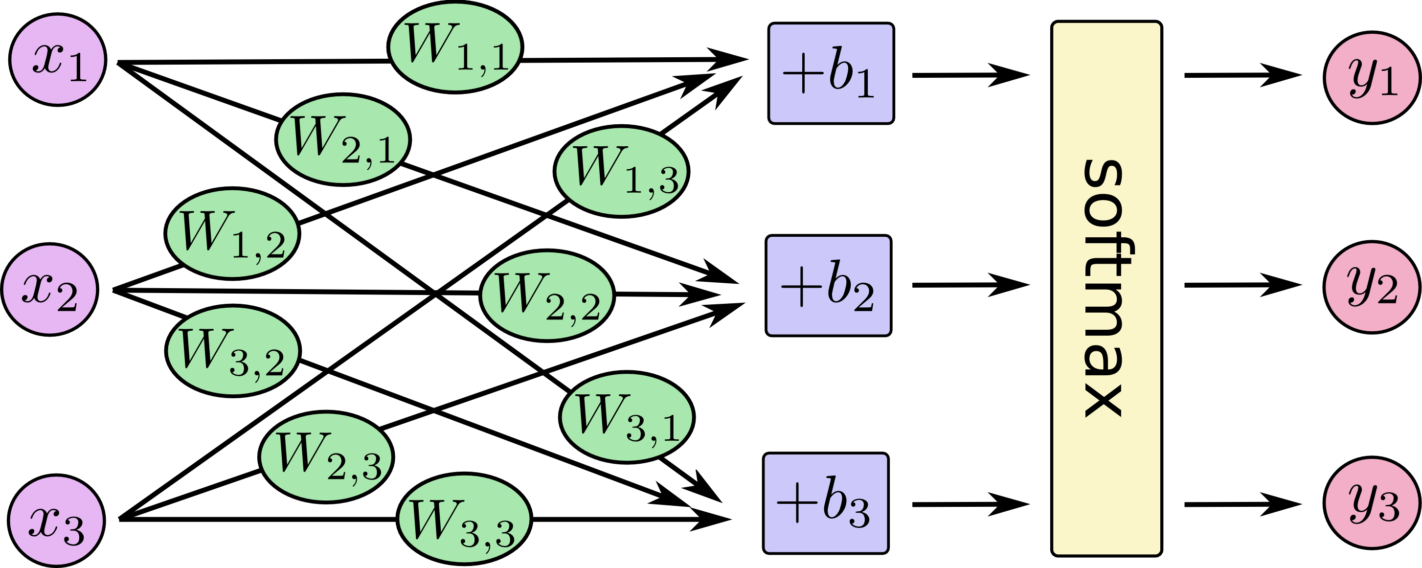
신경망 계산 및 softmax 함수 동작 방식
TensorFlow에서 다음 코드를 입력한다.
from tensorflow.examples.tutorials.mnist import input_data
mnist = input_data.read_data_sets("MNIST_data/", one_hot=True)
import tensorflow as tf
x = tf.placeholder(tf.float32, [None, 784])
W = tf.Variable(tf.zeros([784, 10]))
b = tf.Variable(tf.zeros([10]))
y = tf.nn.softmax(tf.matmul(x, W) + b)
y_ = tf.placeholder(tf.float32, [None, 10])
cross_entropy = tf.reduce_mean(-tf.reduce_sum(y_ * tf.log(y), reduction_indices=[1]))
train_step = tf.train.GradientDescentOptimizer(0.5).minimize(cross_entropy)
sess = tf.InteractiveSession()
tf.global_variables_initializer().run()
for _ in range(1000):
batch_xs, batch_ys = mnist.train.next_batch(100)
sess.run(train_step, feed_dict={x: batch_xs, y_: batch_ys})
correct_prediction = tf.equal(tf.argmax(y,1), tf.argmax(y_,1))
accuracy = tf.reduce_mean(tf.cast(correct_prediction, tf.float32))
print(sess.run(accuracy, feed_dict={x: mnist.test.images, y_: mnist.test.labels}))
이 코드의 실행결과는 다음과 같다. 대략 92% 정확도를 가진 훈련모델을 얻을 수 있다.

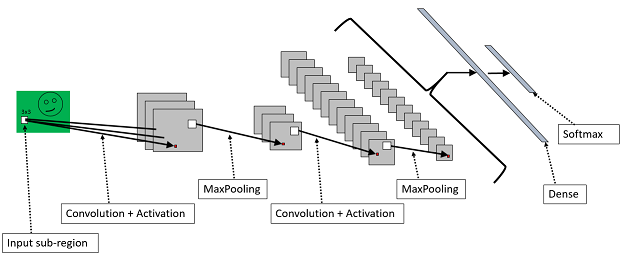
2. CNN 기반 MNIST 훈련
92% 정확도도 나쁘지는 않지만, 99.2% 수준으로 훈련모델을 개선할 수 있는 더 좋은 방법이 있다. CNN(convolutional neural network) 딥러닝을 이용해 다음과 같이 개선한다.
def weight_variable(shape):
initial = tf.truncated_normal(shape, stddev=0.1)
return tf.Variable(initial)
def bias_variable(shape):
initial = tf.constant(0.1, shape=shape)
return tf.Variable(initial)
def conv2d(x, W):
return tf.nn.conv2d(x, W, strides=[1, 1, 1, 1], padding='SAME')
def max_pool_2x2(x):
return tf.nn.max_pool(x, ksize=[1, 2, 2, 1],
strides=[1, 2, 2, 1], padding='SAME')
W_conv1 = weight_variable([5, 5, 1, 32])
b_conv1 = bias_variable([32])
x_image = tf.reshape(x, [-1,28,28,1])
h_conv1 = tf.nn.relu(conv2d(x_image, W_conv1) + b_conv1)
h_pool1 = max_pool_2x2(h_conv1)
W_conv2 = weight_variable([5, 5, 32, 64])
b_conv2 = bias_variable([64])
h_conv2 = tf.nn.relu(conv2d(h_pool1, W_conv2) + b_conv2)
h_pool2 = max_pool_2x2(h_conv2)
W_fc1 = weight_variable([7 * 7 * 64, 1024])
b_fc1 = bias_variable([1024])
h_pool2_flat = tf.reshape(h_pool2, [-1, 7*7*64])
h_fc1 = tf.nn.relu(tf.matmul(h_pool2_flat, W_fc1) + b_fc1)
keep_prob = tf.placeholder(tf.float32)
h_fc1_drop = tf.nn.dropout(h_fc1, keep_prob)
W_fc2 = weight_variable([1024, 10])
b_fc2 = bias_variable([10])
y_conv = tf.matmul(h_fc1_drop, W_fc2) + b_fc2
cross_entropy = tf.reduce_mean(
tf.nn.softmax_cross_entropy_with_logits(labels=y_, logits=y_conv))
train_step = tf.train.AdamOptimizer(1e-4).minimize(cross_entropy)
correct_prediction = tf.equal(tf.argmax(y_conv,1), tf.argmax(y_,1))
accuracy = tf.reduce_mean(tf.cast(correct_prediction, tf.float32))
sess.run(tf.global_variables_initializer())
for i in range(20000):
batch = mnist.train.next_batch(50)
if i%100 == 0:
train_accuracy = accuracy.eval(feed_dict={
x:batch[0], y_: batch[1], keep_prob: 1.0})
print("step %d, training accuracy %g"%(i, train_accuracy))
train_step.run(feed_dict={x: batch[0], y_: batch[1], keep_prob: 0.5})
print("test accuracy %g"%accuracy.eval(feed_dict={
x: mnist.test.images, y_: mnist.test.labels, keep_prob: 1.0}))

3. Fully Connected Feed
MNIST는 머신러닝의 전통적인 문제를 보여준다. 이 챕터에서는 tensorflow sample에 포함되어 있는 fully conntected feed 예제를 실행해 본다. 아나콘다를 설치한 경우, 이 예제는 [아나콘다 설치 폴더]\envs\tensorflow\Lib\site-packages\tensorflow\examples\tutorials에 포함되어 있다.
python fully_connected_feed.py
그럼, 다음과 같은 결과를 얻을 수 있다.

4. TensorBoard 활용 그래프 가시화
텐서보드(TensorBoard)를 이용하면, 텐서플로우 학습모델링 그래프를 시각적으로 확인할 수 있다. 텐서보드를 이용하려면, 텐서보드 그래프 가시화에 필요한 로그 데이터를 저장할 폴더를 지정해야 한다. 다음과 같이 아나콘다에서 텐서보드 logdir를 지정한다.
tensorboard --logdir=[Tensorboard log directory]
예) tensorboard --logdir=d:\program\anaconda3\envs\tensorflow\tensorboard_log
여기에서는 앞의 fully_connected_feed.py 에서 실행된 logdir 폴더에 저장된 데이터를 다음과 같이 텐서보드로 확인해 보겠다.
tensorboard --logdir=/tmp/tensorflow/mnist/logs/fully_connected_feed

실행 후에 다음과 같이, http://localhost:6006/에서 학습된 결과들을 확인할 수 있다.

텐서보드의 그래프를 살펴보면, 학습모델을 어떻게 구성했는 지 직관적으로 파악 수 있다.


fully_connected_feed 텐서플로우 그래프

텐서보드의 임베딩 벡터 가시화
텐서보드의 임베딩 벡터 가중치 T-SINE 가시화 영상(iteration)
지금까지 텐서플로우를 이용해, MNIST를 딥러닝해보고, 학습모델링된 그래프를 가시화해 보는 텐서보드를 살펴보았다. 앞으로, 텐서플로우와 같은 머신러닝 플랫폼을 이용해, 많은 문제들이 지능화되리라 생각한다.
기타 레퍼런스
텐서 플로우 의 텐서 보드 에서 임베딩 벡터 가시화 로 결과 된 데이터 베이스 를 찾아 볼수 있는 가요 ?
답글삭제