이 글은 패션 이미지 데이터를 활용한 PyTorch 기반 모델 훈련 및 예측 방법을 간단히 나눔한다.
파이토치(Pytorch)는 파이썬기반 오픈 소스 머신러닝 라이브러리로 페이스북 인공지능 연구소에 의해 개발되었다. 파이토치는 NVIDIA의 GPU로 병렬처리가 가능해, 높은 실행 성능을 가진다. 토치 사용방법은 Keras와 유사하나, 좀 더 간단히 신경망을 정의하고, 지원되는 유틸리티 사용이 편리하다. 이 글은 패션 이미지를 MNIST처럼 공유한 데이터를 사용해 학습 및 예측을 진행하고, 이를 설명한다.
PyTorch 설치 방법
여러가지 설치 방법이 있으나, 여기서는 anaconda를 사용하기로 한다. pytorch 설치 전에 아래를 참고해, NVIDIA DRIVER, CUDA, 텐서플로우 등을 설치해야 한다. 참고로, 운영체제 환경에 따라 설치 방법은 약간 다를 수 있다.
아래 명령으로 토치를 설치한다.
conda install -c pytorch pytorch
참고로, CUDA 버전에 따라 설치되는 패키지 버전 의존성이 달라져 에러가 발생할 수도 있다. 이 경우는 정답이 없어, 구글링하면서 솔류션을 찾아야 한다.
FashionMNIST 학습 및 예측
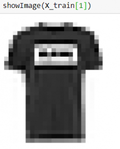
FashionMNIST는 아래와 같은 패션 데이터이다.
라벨은 다음과 같다.


 모델 훈련은 이러한 과정을 반복해 가중치와 바이어스를 조정하는 수치 계산 과정일 뿐이다.
Label Description0 T-shirt/top1 Trouser2 Pullover3 Dress4 Coat5 Sandal6 Shirt7 Sneaker8 Bag9 Ankle boot
아래 코드를 입력하고, 실행해본다.
# 라이브러리 임포트
import torch
from torch import nn
from torch.utils.data import DataLoader
from torchvision import datasets
from torchvision.transforms import ToTensor, Lambda, Compose
import matplotlib.pyplot as plt
# 패션 MNIST 훈련용 데이터셋을 다운로드한다.
training_data = datasets.FashionMNIST(
root="data",
train=True,
download=True,
transform=ToTensor(),
)
# 테스트 데이터를 다운로드한다.
test_data = datasets.FashionMNIST(
root="data",
train=False,
download=True,
transform=ToTensor(),
)
batch_size = 64 # 배치크기 설정
# 데이터 로더 생성
train_dataloader = DataLoader(training_data, batch_size=batch_size)
test_dataloader = DataLoader(test_data, batch_size=batch_size)
for X, y in test_dataloader:
print("Shape of X [N, C, H, W]: ", X.shape)
print("Shape of y: ", y.shape, y.dtype)
break
# 학습용 디바이스 정보 획득
device = "cuda" if torch.cuda.is_available() else "cpu"
print("Using {} device".format(device))
# 모델 정의
class NeuralNetwork(nn.Module):
def __init__(self):
super(NeuralNetwork, self).__init__()
self.flatten = nn.Flatten()
self.linear_relu_stack = nn.Sequential(
nn.Linear(28*28, 512),
nn.ReLU(),
nn.Linear(512, 512),
nn.ReLU(),
nn.Linear(512, 10),
nn.ReLU()
)
def forward(self, x):
x = self.flatten(x)
logits = self.linear_relu_stack(x)
return logits
# 모델 학습을 위한 디바이스 설정
model = NeuralNetwork().to(device)
print(model)
# 모델 학습 솔류션 수렴을 위한 최적화 모델 정의
loss_fn = nn.CrossEntropyLoss()
optimizer = torch.optim.SGD(model.parameters(), lr=1e-3)
# 훈련 함수 정의
def train(dataloader, model, loss_fn, optimizer):
size = len(dataloader.dataset)
for batch, (X, y) in enumerate(dataloader):
X, y = X.to(device), y.to(device)
# Compute prediction error
pred = model(X)
loss = loss_fn(pred, y)
# Backpropagation
optimizer.zero_grad()
loss.backward()
optimizer.step()
if batch % 100 == 0:
loss, current = loss.item(), batch * len(X)
print(f"loss: {loss:>7f} [{current:>5d}/{size:>5d}]")
# 테스트 함수 정의
def test(dataloader, model):
size = len(dataloader.dataset)
model.eval()
test_loss, correct = 0, 0
with torch.no_grad():
for X, y in dataloader:
X, y = X.to(device), y.to(device)
pred = model(X)
test_loss += loss_fn(pred, y).item()
correct += (pred.argmax(1) == y).type(torch.float).sum().item()
test_loss /= size
correct /= size
print(f"Test Error: \n Accuracy: {(100*correct):>0.1f}%, Avg loss: {test_loss:>8f} \n")
epochs = 10 # 학습을 원하는 만큼 수정요
for t in range(epochs):
print(f"Epoch {t+1}\n-------------------------------")
train(train_dataloader, model, loss_fn, optimizer)
test(test_dataloader, model)
print("Done!")
# 모델 학습 가중치 파일 저장
torch.save(model.state_dict(), "model.pth")
print("Saved PyTorch Model State to model.pth")
# 가중치 파일을 통한 모델 로드
model = NeuralNetwork()
model.load_state_dict(torch.load("model.pth"))
# 예측을 위한 클래스 정의
classes = [
"T-shirt/top",
"Trouser",
"Pullover",
"Dress",
"Coat",
"Sandal",
"Shirt",
"Sneaker",
"Bag",
"Ankle boot",
]
# 모델 평가
model.eval()
x, y = test_data[0][0], test_data[0][1]
with torch.no_grad():
pred = model(x) # 패션 MNIST 데이터 입력 후 예측
predicted, actual = classes[pred[0].argmax(0)], classes[y]
print(f'Predicted: "{predicted}", Actual: "{actual}"')
실행 결과는 다음과 같다.
/home/ktw/anaconda3/envs/pytorch/bin/python /home/ktw/.local/share/JetBrains/Toolbox/apps/PyCharm-C/ch-0/211.6693.115/plugins/python-ce/helpers/pydev/pydevd.py --multiproc --qt-support=auto --client 127.0.0.1 --port 39301 --file /home/ktw/Projects/pytorch/MNIST.py
Connected to pydev debugger (build 211.6693.115)
Backend Qt5Agg is interactive backend. Turning interactive mode on.
Shape of X [N, C, H, W]: torch.Size([64, 1, 28, 28])
Shape of y: torch.Size([64]) torch.int64
Using cuda device
NeuralNetwork(
(flatten): Flatten(start_dim=1, end_dim=-1)
(linear_relu_stack): Sequential(
(0): Linear(in_features=784, out_features=512, bias=True)
(1): ReLU()
(2): Linear(in_features=512, out_features=512, bias=True)
(3): ReLU()
(4): Linear(in_features=512, out_features=10, bias=True)
(5): ReLU()
)
)
Epoch 1
-------------------------------
loss: 2.299011 [ 0/60000]
loss: 2.295951 [ 6400/60000]
loss: 2.283560 [12800/60000]
loss: 2.278397 [19200/60000]
loss: 2.284869 [25600/60000]
loss: 2.267760 [32000/60000]
loss: 2.266866 [38400/60000]
loss: 2.257998 [44800/60000]
loss: 2.237380 [51200/60000]
loss: 2.209423 [57600/60000]
Test Error:
Accuracy: 41.4%, Avg loss: 0.034879
...
est Error:
Accuracy: 57.0%, Avg loss: 0.022959
Done!
Saved PyTorch Model State to model.pth
Predicted: "Sneaker", Actual: "Ankle boot"
이제 학습 반복 세대를 높여서 실행해보자. 세대를 10으로 수정한 후 loss는 0.018335로 줄었음을 확인할 수 있다.

파이토치 기능 및 모델구조 설명
토치는 데이터 로딩 작업을 위해, torch.utils.data.DataLoader, torch.utils.data.Dataset을 제공한다. torchvision.datasets 모듈은 CIFAR, COCO 등 유명한 데이터셋 로딩을 지원한다.
앞의 소스에서 배치 크기는 64이므로, 데이터로더의 iterator는 64개의 이미지와 레이블을 반환하게 된다.
모델 정의는 다음과 같다.
class NeuralNetwork(nn.Module):
def __init__(self):
super(NeuralNetwork, self).__init__()
self.flatten = nn.Flatten()
self.linear_relu_stack = nn.Sequential(
nn.Linear(28*28, 512),
nn.ReLU(),
nn.Linear(512, 512),
nn.ReLU(),
nn.Linear(512, 10),
nn.ReLU()
)
def forward(self, x):
x = self.flatten(x)
logits = self.linear_relu_stack(x)
return logits
토치의 상위 클래스, nn.Module을 파생받은 NeuralNetwork 클래스를 정의해야 한다(Torch.NN 참고).

UML(lucid.app)
생성자에서 모델을 정의한다. nn은 신경망 구조를 제공한다. nn.ReLU는 비선형 학습 활성화 함수를 정의한다. flatten은 주어진 2차원 벡터 이미지를 1차원으로 벡터로 변환한다.
nn.Sequential은 정의된 순서대로 데이터가 전달되도록 하는 컨테이너이다. 이 컨테이너에 신경망 구조를 순서대로 정의하면 된다. 모델링된 결과는 다음과 같다. 28x28 이미지(784 픽셀)는 Linear 레이어로 입력되어, 512 출력노드로 맵핑된다. 이 레이어의 출력값은 ReLU로 전달되고, 다시 Linear 레이어로 512 출력노드로 맵핑되어 ReLU로 변환된다. 이 결과는 다시 10개의 출력노드를 가진 Linear 레이어로 맵핑되고 ReLU로 변환된다.
NeuralNetwork(
(flatten): Flatten(start_dim=1, end_dim=-1)
(linear_relu_stack): Sequential(
(0): Linear(in_features=784, out_features=512, bias=True)
(1): ReLU()
(2): Linear(in_features=512, out_features=512, bias=True)
(3): ReLU()
(4): Linear(in_features=512, out_features=10, bias=True)
(5): ReLU()
)
)
역전파 알고리즘 함수는 토치에서 train의 forward함수를 이용해 자동으로 생성해준다.
역전파 알고리즘은 신경망의 입력층과 출력층의 차이를 조정하기 위해, 가중치를 얼마나 보정해야 하는 지를 계산한다. 이 보정치는 손실함수의 기울기값이라고 말하며, 이는 다음 그림에서 신경망 가중치와 바이어스를 기울기 값으로 수정할때 사용된다. 손실함수는 계산된 결과와 목표값의 차이를 계산하여, 이 차이값을 최소화할 때 사용된다.
앞의 소스에서는 학습 파라메터인 파이퍼 파라메터를 다음과 같이 설정했었다.
learning_rate = 1e-3
batch_size = 64
epochs = 5
여기서 learning_rate는 옵티마이저에 설정되는 학습률이다.
옵티마이저는 각 학습 단계에서 모델 오류를 줄이기 위해 모델 손실값을 조정해 나간다. SDG는 확률기반 경사 하강법이며, 토치에는 이외 다양한 최적화 함수가 있다. 모델의 파라메터를 통해 최적화 함수는 모델 구조, 파라메터, 역전파 함수를 얻어 이를 최적화할 때 사용한다.
optimizer = torch.optim.SGD(model.parameters(), lr=learning_rate)
결국, 다음과 같이 앞에서 정의한 데이터 로딩 방법, 모델, 손실 함수, 최적화 함수를 이용해 세대별로 반복 학습을 하게 된다.
for t in range(epochs):
print(f"Epoch {t+1}\n-------------------------------")
train(train_dataloader, model, loss_fn, optimizer)
test(test_dataloader, model)
훈련된 모델은 파일로 저장해 필요할 때 로딩해 사용할 수 있다. ONNX(Open Neural Network Exchange) 로딩 및 저장도 함께 제공한다.
모델 구조 수정 후 결과 비교
모델 구조를 수정해 결과를 확인해 보자. 참고로, 원래 소스 결과는 5세대 훈련 시 Accuracy: 57.0%, Avg loss: 0.022959 였다.
1. 2개 은닉층
NeuralNetwork(
(flatten): Flatten(start_dim=1, end_dim=-1)
(linear_relu_stack): Sequential(
(0): Linear(in_features=784, out_features=512, bias=True)
(1): ReLU()
(2): Linear(in_features=512, out_features=10, bias=True)
(3): ReLU()
)
)
Test Error:
Accuracy: 33.4%, Avg loss: 0.030179
Done!
Saved PyTorch Model State to model.pth
Predicted: "Ankle boot", Actual: "Ankle boot"
2. 4개 은닉층
NeuralNetwork(
(flatten): Flatten(start_dim=1, end_dim=-1)
(linear_relu_stack): Sequential(
(0): Linear(in_features=784, out_features=512, bias=True)
(1): ReLU()
(2): Linear(in_features=512, out_features=512, bias=True)
(3): ReLU()
(4): Linear(in_features=512, out_features=512, bias=True)
(5): ReLU()
(6): Linear(in_features=512, out_features=10, bias=True)
(7): ReLU()
)
)
Test Error:
Accuracy: 38.2%, Avg loss: 0.032565
Done!
Saved PyTorch Model State to model.pth
Predicted: "Ankle boot", Actual: "Ankle boot"
3. 4개 은닉층에서 입출력을 512-256으로 매핑.
NeuralNetwork(
(flatten): Flatten(start_dim=1, end_dim=-1)
(linear_relu_stack): Sequential(
(0): Linear(in_features=784, out_features=512, bias=True)
(1): ReLU()
(2): Linear(in_features=512, out_features=512, bias=True)
(3): ReLU()
(4): Linear(in_features=512, out_features=256, bias=True)
(5): ReLU()
(6): Linear(in_features=256, out_features=10, bias=True)
(7): ReLU()
)
)
Test Error:
Accuracy: 39.7%, Avg loss: 0.032889
Done!
Saved PyTorch Model State to model.pth
Predicted: "Ankle boot", Actual: "Ankle boot"
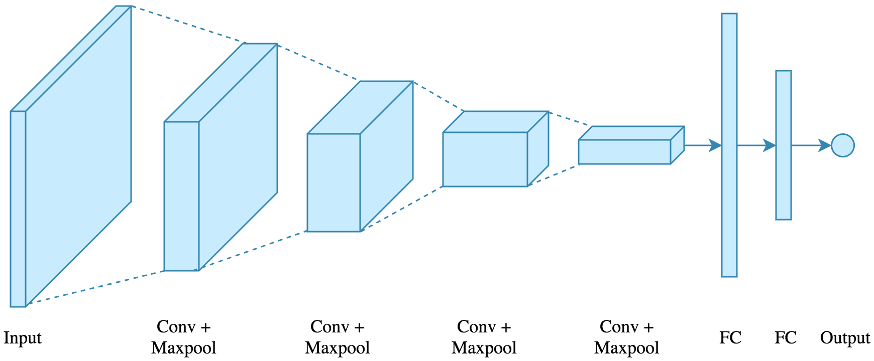
결과와 같이 모델 구조에 따라 정확도 및 손실률이 달라진다. 이 모델은 CNN을 사용하지 않았다. 다음과 같이 CNN 모델을 사용할 경우, 정확도는 매우 높아진다.
CNN 모델은 다음과 같이 정의한다.
x = Image(28 * 28 * 1) # 그레이컬러 입력채널 1개, 이미지 크기 28 x 28
x = x * Conv2d(1, 8, 3) # 입력채널 1개, 출력(필터)채널 8개, 커널크기 3
x = ReLu(x)
x = Pooling(x)
x = x* Conv2d(8, 16, 3) # 입력채널 8개, 출력채널 16개, 커널크기 3
x = ReLu(x)
x = Pooling(x)
x = Reshape(x, -1, 7 * 7 * 16)
x = Dropout(ReLu(Linear(x, 28 * 28, 16 * 16))) # 입력 이미지 28 x 28, 출력 256
x = Dropout(ReLu(Linear(x, 16 * 16, 128)))
x = Dropout(ReLu(Linear(x, 128, 8 * 8)))
x = Linear(x, 8 * 8, 10)
코드 구현은 다음과 같다.
class Net(nn.Module):
def __init__(self):
super(Net, self).__init__()
# convolutional layers
self.conv1 = nn.Conv2d(1, 8, 3, padding=1)
self.conv2 = nn.Conv2d(8, 16, 3, padding=1)
# linear layers
self.fc1 = nn.Linear(784, 256)
self.fc2 = nn.Linear(256, 128)
self.fc3 = nn.Linear(128, 64)
self.fc4 = nn.Linear(64, 10)
# dropout
self.dropout = nn.Dropout(p=0.2)
# max pooling
self.pool = nn.MaxPool2d(2, 2)
def forward(self, x):
# convolutional layers with ReLU and pooling
x = self.pool(F.relu(self.conv1(x)))
x = self.pool(F.relu(self.conv2(x)))
# flattening the image
x = x.view(-1, 7 * 7 * 16) # reshape
# linear layers
x = self.dropout(F.relu(self.fc1(x)))
x = self.dropout(F.relu(self.fc2(x)))
x = self.dropout(F.relu(self.fc3(x)))
x = self.fc4(x)
return x
이 경우, 정확도는 평균 77.31%로 높아진다. 레이어가 깊다고 정확도가 높아지는 것은 아니다. 실제 Conv2d(64, 32) 층을 하나 더 추가하고 학습하면 정확도가 67.19%로 오히려 떨어지는 현상을 볼 수 있다.
다음과 같이 레이어를 하나 더 줄이고 테스트하면 오히려 정확도가 79.98%로 높아진다. 정확도는 학습 데이터 수, 품질, 학습 횟수 등 모델 구조 이외 다른 요소들도 영향을 주므로, 이런 부분은 경험적으로 모델을 설계해야 한다.
lass Net(nn.Module):
def __init__(self):
super(Net, self).__init__()
# convolutional layers
self.conv1 = nn.Conv2d(1, 8, 3, padding=1)
self.conv2 = nn.Conv2d(8, 16, 3, padding=1)
# linear layers
self.fc1 = nn.Linear(784, 256)
self.fc2 = nn.Linear(256, 96)
self.fc3 = nn.Linear(96, 10)
# dropout
self.dropout = nn.Dropout(p=0.2)
# max pooling
self.pool = nn.MaxPool2d(2, 2)
def forward(self, x):
# convolutional layers with ReLU and pooling
x = self.pool(F.relu(self.conv1(x)))
x = self.pool(F.relu(self.conv2(x)))
# flattening the image
x = x.view(-1, 7 * 7 * 16)
# linear layers
x = self.dropout(F.relu(self.fc1(x)))
x = self.dropout(F.relu(self.fc2(x)))
x = self.fc3(x)
return x
적절한 모델 구조를 찾는 것은 시행착오가 필요하다. 적절한 모델을 찾는 것을 Fitting 한다고 한다. 참고로, AutoML, Model Search같은 라이브러리를 사용하면, 앞서 정의한 모델을 자동으로 얻을 수 있다(AutoML tutorial).
참고 - 토치 지원 모델
토치에서 지원하는 기타 모델 및 사용 예시는 다음과 같다(참고).
- Containers
- Convolution Layers
- Pooling layers
- Padding Layers
- Non-linear Activations (weighted sum, nonlinearity)
- Non-linear Activations (other)
- Normalization Layers
- Recurrent Layers
- Transformer Layers
- Linear Layers
- Dropout Layers
- Sparse Layers
- Distance Functions
- Loss Functions
- Vision Layers
- Shuffle Layers
- DataParallel Layers (multi-GPU, distributed)
- Utilities
- Quantized Functions
- Lazy Modules Initialization
사용 예시.
>>> rnn = nn.LSTM(10, 20, 2)
>>> input = torch.randn(5, 3, 10)
>>> h0 = torch.randn(2, 3, 20)
>>> c0 = torch.randn(2, 3, 20)
>>> output, (hn, cn) = rnn(input, (h0, c0))
참고: 케라스와 모델 정의 차이점
케라스는 모델 정의 방법이 다음과 같이 좀 더 상세하다. 토치는 이에 비해 간략하게 모델을 정의할 수 있다.
model = Sequential()
model.add(Dense(1024, input_shape=(3072,), activation="sigmoid"))
model.add(Dense(512, activation="sigmoid"))
model.add(Dense(len(lb.classes_), activation="softmax"))
...
model = tf.keras.models.Sequential([
tf.keras.layers.Flatten(input_shape=(28, 28)),
tf.keras.layers.Dense(128,activation='relu'),
tf.keras.layers.Dense(10)
])
...
model = Sequential()
model.add(LSTM(4, input_shape=(1, look_back)))
model.add(Dense(1))
model.compile(loss='mean_squared_error', optimizer='adam')
model.fit(trainX, trainY, epochs=100, batch_size=1, verbose=2)
이외 토치는 케라스보다 실행 성능이 빠르고 확장성이 좋다고 알려져 있다.
레퍼런스
- PyTorch Quick start
- PyTorch Tutorial
- PyTorch 사용법
- PyTorch 모델 정의
- How to Perform Classification with AutoML
- Automated Machine Learning Libraries for Python and tutorial
- AutoML Vision API
- Keras Tutorial
- PyTorch Tutorial (Korean) (last)
- Fashion MNIST using CNN (github)
- Pytorch [Basics] — Intro to CNN
- CNN summary
- Keras CNN understanding
Thanks for sharing a very informative article! If you are looking for the best Node JS Development Services then visit us now.
답글삭제Thanks.
삭제