Daddy Makers: 4월 2024

2024년 4월 26일 금요일

공간정보 GIS 기반 IoT 데이터 분석 스타일 데쉬보드 만들고 서비스해보기

이 글은 Django, Bootstrap을 사용해 GIS 기반 IoT 데이터 분석 스타일의 데쉬보드 개발방법을 간략히 정리하고, 개발 방법 후 서비스하는 방법을 보여준다. 이를 통해, 공간정보 기반 IoT 장비를 하나의 데쉬보드로 관리하고, 분석하는 것이 가능하다. 여기서 공간정보는 GIS, BIM, 3D Point cloud data 와 같이 공간상 좌표로 표현되는 모든 정보를 말한다. 상세한 구현 소스 코드는 본 글의 Github링크를 참고할 수 있다.

IoT 데쉬보드 web app 서버 실행 (example)

이 글을 통해, 다음 내용을 이해할 수 있다.

부트스트랩 데쉬보드 UI 라이브러리 사용법
장고의 데이터 모델과 웹 UI 간의 연계 방법
GIS 맵 가시화 및 이벤트 처리
실시간 IoT 데이터에 대한 동적 UI 처리 방법

이 글의 독자는 장고, 부트스트랩, GIS, IoT 의 기본 개념은 알고 있다고 가정한다.

요구사항 디자인

다음과 같은 목적의 웹앱 서비스를 가정한다.

GIS 기반 센서 위치 관리
IoT 데이터셋 표현
IoT 장치 관리
IoT 장치 활성화 관리 KPI 표현
계정 관리
기타 메뉴

이러한 정보를 보여줄 수 있는 데쉬보드 웹앱을 디자인한다. 이 예제는 데쉬보드 레이아웃을 가진 웹앱 프레임 개발 방법을 보여주는 것에 집중한다. 세부 비지니스 로직 및 데이터베이스 모델은 다른 페이지를 참고한다.

개발환경 준비

개발도구

개발에 필요한 도구는 다음으로 한다.

UI: bootstrap
웹앱 프레임웍: DJango
GIS: leaflet, Cesium
데이터소스: sqlite, spreadsheet, mongodb

구현된 상세 소스코드는 다음을 참고한다.

mac999/IoT_simple_dashboard: IoT simple dashboard (github.com)

장고 기반 웹앱 프로젝트 생성

장고(Django)는 파이썬으로 작성된 고수준의 웹 프레임워크로, 웹 애플리케이션 개발을 빠르고 쉽게 할 수 있도록 도와준다. 장고는 "The web framework for perfectionists with deadlines"라는 슬로건을 가지고 있으며, 많은 기능을 내장하고 있어 개발자가 반복적인 작업을 줄이고 핵심 기능에 집중할 수 있도록 한다.

다음과 같이 장고 웹앱 프로젝트를 생성한다.

python -m venv myenv

source myenv/bin/activate

pip install django pandas

django-admin startproject iot_dashboard

cd iot_dashboard

python manage.py startapp dashboard

생성된 프로젝트 폴더 구조는 다음과 같다.

디자인 스타일 고려사항

부트스랩 레이아웃 표현

부트스트랩(Bootstrap)은 웹 개발에서 널리 사용되는 프론트엔드 프레임워크로 주로 HTML, CSS, JavaScript로 작성되어 있다. 트위터의 개발자들에 의해 처음 만들어졌으며, 웹 애플리케이션의 개발 속도를 높이고, 반응형 디자인을 쉽게 구현할 수 있도록 도와준다.

부트스랩의 그리드 시스템은 12개 열로 디자인된다. 이는 유연성과 사용 편의성을 제공하기 위한 디자인 결정이다. 반응형 웹사이트를 구축하는 데 많이 사용된다.

참고로, 12라는 숫자는 많은 약수(1, 2, 3, 4, 6, 12)를 갖고 있어 다양한 열의 조합으로 균등하게 나눌 수 있다. 이를 통해 분수나 번거로운 나머지 없이 다양한 레이아웃을 만들 수 있다.

유연성: 12개의 열을 사용하면 다양한 화면 크기와 디바이스에 적합한 레이아웃을 쉽게 만들 수 있다. 각 요소가 차지하는 열의 수를 조정하여 대형 데스크톱 화면, 태블릿 및 스마트폰에서 잘 보이는 반응형 디자인을 만들 수 있다.
이해하기 쉬움: 12개의 열을 기반으로 한 그리드 시스템은 디자이너와 개발자들에게 직관적이다. 그리드 내에서 요소들이 어떻게 동작할지 시각화하고 계산하기 쉽기 때문에 일관된 레이아웃을 생성하고 유지하기가 간단하다.
디자인 관행: 12개의 열을 사용하는 그리드 시스템은 부트스트랩 이전부터 다양한 그래픽 디자인 및 레이아웃 소프트웨어에서 사용되어 왔다.

데쉬보드 카드 스타일

데쉬보드에 컨텐츠를 담을 패널을 카드 스타일로 표현할 수 있다. 카드 내에 차트 뿐 아니라 지도 등 그래픽도 표시할 수 있다.

Bootstrap Cards - free examples & easy customization (mdbootstrap.com)

보통, 일반적인 카드 스타일 구조는 다음과 같다.

<i class="fa fa-map"></i> Leaflet Map

</div>

</div>

이 코드는 행 스타일 안에 가변 8개 컬럼을 차지(col-lg-8)하고, 중간 수준 마진(card mb-3)를 가지는 카드를 생성한다. 카드는 헤더(card_header)와 본체(card-body)를 가지며, 헤더는 아이콘(<i>) 스타일의 Font Awesome의 map 아이콘을 사용한다. body 내에는 디스플레이할 위젯을 표시할 <div>를 정의한다.

부트스랩은 이와 같은 style tag가 있어, 다양한 UI를 손쉽게 정의할 수 있다. 자세한 내용은 다음을 참고한다.

Introduction · Bootstrap (getbootstrap.com)

개발

주요 구현부분만 표현한다. 상세 구현 코드는 앞의 github 링크를 참고한다.

데이터소스 모델 연결 및 차트 표시

본 예시는 데쉬보드 앱 디자인 및 개발 과정을 보여주는 것이므로, 간단한 iot sample dataset을 다음과 같이 models.py에 개발해 놓는다.

def IoT_model_from_file():

save_sample_iot_dataset()

df = pd.read_csv('iot_dataset_sample.csv')

json_dict = df.to_dict('records')

return json_dict

def save_sample_iot_dataset():

# Create a DataFrame

df = pd.DataFrame({

'time': [datetime.now() - timedelta(days=i) for i in range(10)],

'open': [randint(100, 200) for _ in range(10)],

'high': [randint(200, 300) for _ in range(10)],

'low': [randint(50, 100) for _ in range(10)],

'close': [randint(100, 200) for _ in range(10)],

})

# Convert the 'time' column to a string in the format 'YYYY-MM-DD'

df['time'] = df['time'].dt.strftime('%Y-%m-%d')

# Save the DataFrame to a CSV file

df.to_csv('iot_dataset_sample.csv', index=False)

IoT 센서 실시간 데이터 표시

특정 카드 내 차트에 실시간으로 데이터를 표현하기 위해서, 장고에서는 html script > view > model 업데이트 과정을 거쳐야 한다. 이 경우는 3초마다 센서 데이터를 화면에 업데이트한다고 가정한다. 이를 위해, 데이터가 준비되면 렌더링될 수 있도록 비동기 처리 요구 방식을 사용한다.

index.html의 script부분에 아래 코드를 추가한다.

setInterval(fetchColumnData, 3000); // 3초마다 업데이트

function fetchColumnData() {

var xhr = new XMLHttpRequest();

xhr.open('GET', '/charts?chartType=column', true);

xhr.onreadystatechange = function () {

if (xhr.readyState == 4 && xhr.status == 200) { // 비동기. 데이터 준비 시 호출

var columnData = JSON.parse(xhr.responseText);

columnChart.options.data[0].dataPoints = columnData;

columnChart.render(); // 값을 차트에 업데이트

var columnChart_ready = document.getElementById('columnChart_ready');

var columnChart_operation = document.getElementById('columnChart_operation');

var columnChart_shutdown = document.getElementById('columnChart_shutdown');

columnChart_ready.innerHTML = columnData[0].y;

columnChart_operation.innerHTML = columnData[1].y;

columnChart_shutdown.innerHTML = columnData[2].y;

}

};

xhr.send();

}

참고로, 이러한 방식은 많은 CPU 부하를 차지한다. 다른 대안으로, 다음처럼 animation loop를 사용하는 방식이 있다.

let lastTime = 0;

const interval = 3000;

function animationLoop(timestamp) {

if (timestamp - lastTime >= interval) {

fetchColumnData();

lastTime = timestamp;

}

requestAnimationFrame(animationLoop);

}

requestAnimationFrame(animationLoop);

이 또한 성능 문제가 있다면, 실시간 업데이트 기능이 필요한 사용자만 사용할 수 있도록 페이지를 분리하거나, 별도 UI 앱을 개발하자.

이외, Leaflet(리플렛), Cesium(세슘) 라이브러리를 이용해 2차원, 3차원 화면을 표시한다. 세귬은 미리 API 사용 토큰을 발급받아야 제대로 동작된다.

Cesium.Ion.defaultAccessToken = 'your_access_token';

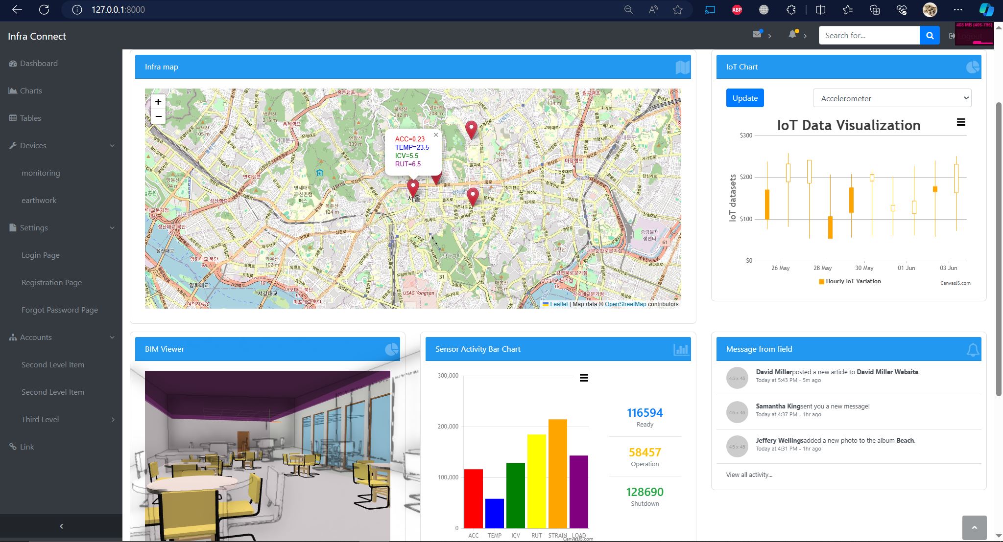
실행 결과

앞의 디자인 목적을 고려한 데쉬보드 실행 결과는 다음과 같다.

번들(buddle)로 컴파일된 자바스크립트 라이브러리 중 하나인 ifc.js의 viewer를 card-body의 id와 연결하여, 다음과 같이 3D 모델을 표현할 수 있다. Cesium도 동일한 방식으로 렌더링될 수 있다.

웹 서비스 배포 및 호스팅

호스팅 방법은 다양하다. 여기에선 최근 인기가 높아지고 있는 cloudtype을 사용해 배포한다.

cloud server setting 모습

배포에 성공하면, 다음과 같이 외부에서도 웹 서비스에 접속 실행될 것이다.

Infra IoT Dashboard server

실행 화면

스마트폰에서 접속하면, bootstrap layout style에 따라 패널이 잘 정렬되어 보여지는 것을 확인할 수 있다.

스마트 폰 실행 모습

이외에 유용한 배포 호스팅 서버로 python anywhere, amazon free tier 등이 있다. 아래 링크를 참고한다.

마무리

요즘에는 좋은 개발 도구와 라이브러리가 워낙 많아, 프론트앤드, 백앤드, 미들웨어 스택을 만들때 조합하기가 오히려 혼란스러운 점이 있다. 장고, 부트스랩 등을 이용하면 기본적인 프레임웍에서 이들을 조합할 수 있어, 개발이 편해진다.

GIS, BIM, 3D Point cloud data 관련 유명한 라이브러리는 CDN 스토리지를 지원하고 있어, import해 사용하기 편하다. 다만, 이런 공간정보 라이브러리는 많은 리소스를 차지하므로, 성능 최적화를 고려해야 사용할 필요가 있다.

추신. 2005년에 개발된 장고는 저널리즘을 전공한 Adrian Holovaty의 주도로 Joscho Stephan과 함께 개발되었다. 그들은 올바른 저널리즘과 기타 연주를 사랑한다.

Django 개발자 Joscho Stephan, Adrian Holovaty (patrus)

레퍼런스

2024년 4월 21일 일요일

LLM 모델 통합과 다양한 데이터소스를 지원하는 LangChain 아키텍처 및 동작 메커니즘 분석하기

이 글은 해리슨 체이스가 개발한 오픈소스인 랭체인(LangChain) 아키텍처와 동작 방법을 분석한다. 현재 개발자들 사이에 대중적으로 사용되고 있는 랭체인은 LLM 모델 통합과 다양한 데이터소스를 지원하여, LLM모델의 활용성을 극대화한다. 이 글을 통해, LLM 서비스 개발에 필요한 랭체인의 아키텍처와 동작 원리를 이해할 수 있다.

LLM 용어와 상세 개념은 다음 링크를 참고한다.

개요

Langchain(랭체인)은 LLM에 원하는 결과를 얻을 수 있도록, 다양한 프롬프트 입력 및 구조화된 출력, RAG, 튜닝과 같은 기능을 제공하는 라이브러리다. 랭체인 설치는 다음과 같다(참고).

pip install langchain

기본 사용법

랭체인은 모델 입출력, 데이터 검색, 에이전트 지원, 체인, 컨텍스트 메모리 기능을 제공하며, LCEL(LangChain Expression Language)를 이용해 각 구성요소를 유기적으로 연결시킬 수 있다. LCEL은 유닉스 파이프라인 개념을 차용했다. 다음은 LCEL 예시를 보여준다.

from langchain.chat_models import ChatOpenAI

from langchain.prompts import ChatPromptTemplate

from langchain.schema import BaseOutputParser

# LCEL 예시

chain = ChatPromptTemplate() | ChatOpenAI() | CustomOutputParser()

이와 더불어, 목적에 맞는 다양한 프롬프트 템플릿, 구조화된 출력을 제공한다.

from langchain.output_parsers.json import SimpleJsonOutputParser

json_prompt = PromptTemplate.from_template(

"Return a JSON object with `birthdate` and `birthplace` key that answers the following question: {question}"

)

json_parser = SimpleJsonOutputParser() # JSON 파서

# 프롬프트, 모델, 파서 체인 생성

json_chain = json_prompt | model | json_parser # 유닉스 파이프라인 개념 차용함.

result_list = list(json_chain.stream({"question": "When and where was Elon Musk born?"}))

print(result_list)

구조 분석

패키지 구조

langchain 구조를 분석하기 위해, github clone 후 UML로 모델링해 본다. 주요 패키지는 다음과 같다.

cli는 langchain의 command line interface, core는 langchain의 핵심 구현 코드가 정의된다. 이 부분은 다음 패키지로 구성된다.

참고로, 이 패키지들은 다음 그림의 일부이다.

Langchain v.0.2.0 패키지

LCEL 언어 동작 구조

이 중에 핵심적인 것만 분석해 본다. 우선, LCEL의 동작 방식을 위해 어떤 디자인패턴을 구현하였는 지 확인한다. 이 부분은 runnables 패키지가 담당한다. 이 언어는 유닉스의 파이프라인 처리를 다음과 같이 흉내낸다.

z = a | b | c

z.stream('abc')

이를 위해, 파이썬 문법을 적극 사용하고 있다. 우선 '|' 연산자를 오버로딩(overloading)하기 위해, 파이썬 Runnable 클래스를 정의해 __or__ 연산자를 구현한다. 이 연산자는 self object와 right object 두 객체를 입력받아 list를 만든 후 리턴하는 역할을 한다. 앞의 예시에서 보면, 'a | b'를 실행가능한 객체 리스트로 만들어 리턴한다. 결론적으로 a, b, c객체를 리스트로 만들고, 이 리스트를 z에 할당한다.

z의 stream()이 호출되면, a, b, c를 각각 invoke() 하여 실행하는 방식이다. 그러므로, 다음 그림과 같이, LCEL를 지원하는 객체는 Runnable을 파생받아야 하며, stream, invoke와 같은 주요 함수를 구현해야 한다.

각 주요 클래스 함수의 동작방식을 좀 더 자세히 살펴본다. LCEL 파이프라인을 구현하는 __or__()함수는 다음과 같이 입력된 객체를 Sequence 형식의 steps 리스트로 담아두는 역할을 한다.

class Runnable():

...

def __or__(self, other: Union[Runnable[Any, Other], Callable[[Any], Other], ...]):

return RunnableSequence(self, coerce_to_runnable(other))

def stream(self, input: Input, config, **kwargs: Optional[Any]) -> Iterator[Output]:

yield self.invoke(input, config, **kwargs) # steam 호출 시 invoke 함수 호출

def invoke(self, input: Input, config: Optional[RunnableConfig] = None):

callback_manager = get_callback_manager_for_config(config)

run_manager = callback_manager.on_chain_start(dumpd(self), input)

for i, step in enumerate(self.steps):

input = step.invoke(input) # steps 리스트의 객체 invoke() 호출 후 input 갱신

invoke()가 호출되면, 담아둔 steps 리스트의 객체를 각각 invoke()한다. 이런 방식으로 파이프라인을 구현하고 있다.

프롬프트 템플릿 처리 방식

JSON과 같이 구조화된 출력을 생성할 때는 ...Template 이름을 가진 클래스가 create_template_from_message_type() 함수를 구현한다. 그 과정을 확인해 보자.

def create_template_from_message_type(message_type, template, template_format):

if message_type in ("human", "user"): # human, user 일 경우, human template 생성

message =HumanTemplate.from_template(template, template_format)

elif message_type in ("ai", "assistant"): # ai 일 경우, AI template 생성

message = AIMessagePromptTemplate.from_template(template, template_format)

elif message_type == "system":

message = SystemMessagePromptTemplate.from_template(...)

elif message_type == "placeholder": # 변수 형태로 출력할 경우, placeholder 생성

if isinstance(template, str):

var_name = template[1:-1]

message = MessagesPlaceholder(variable_name=var_name, optional=True)

elif len(template) == 2 and isinstance(template[1], bool):

var_name = var_name_wrapped[1:-1]

message = MessagesPlaceholder(variable_name=var_name, optional=is_optional)

프롬프트 템플릿에 따라 적절한 템플릿 객체를 생성해 처리한다. invoke() 했을 때, input에 대한 각각 적합한 프롬프트를 출력한다.

변수가 담긴 출력을 위해서는 메시지에서 변수를 예측해야 한다. 이 부분은 from_messages_and_schema()가 담당한다.

def from_messages_and_schema(messages, schema):

# 자동적으로 메시지로 부터 변수를 추정함

input_vars: Set[str] = set()

partial_vars: Dict[str, Any] = {}

for _message in _messages:

if isinstance(_message, MessagesPlaceholder) and _message.optional:

partial_vars[_message.variable_name] = []

elif isinstance(

_message, (BaseChatPromptTemplate, BaseMessagePromptTemplate)

input_vars.update(_message.input_variables) # 변수값 업데이트

출력 텍스트에서 구조화된 출력을 위해, 변수와 변수 유형을 검증해야 한다. 이 기능은 PyDantic을 이용해 처리한다.

앞서 정의된 클래스는 LLM에 입력할 프롬프트를 작성하고, 출력된 결과를 파싱하는 것에 초점을 맞추고 있다.

LLM 모델 호출과 임베딩 데이터베이스 처리

LLM 처리 부분은 llm.py, llms.py 소스에 구현되어 있다. Chain은 전문가가 질문에 답변하며 정보를 업데이트하는 연속된 질의를 담당한다. BaseLLM은 LLM 이 호출될 수 있도록 일반화한 클래스이다. invoke()가 호출되면 프롬프트, 입력과 함께 _agenerate()이 호출된다. 이 함수는 실제 설치된 라마와 같은 LLM혹은 OpenAI의 ChatGPT API를 호출해 출력을 생성하는 역할을 한다.

class LLMChain(Chain):

async def _agenerate(self, prompts: List[str], ..., **kwargs: Any) -> LLMResult:

class BaseLLM():

async def _agenerate(self, prompts: List[str], ..., **kwargs: Any) -> LLMResult:

return await run_in_executor(None, self._generate, prompts, stop, ..., **kwargs)

LangChain은 임베딩 벡터 데이터베이스를 지원함으로써 LlamaIndex와 함께 RAG를 처리한다. 이를 통해, 환각 현상을 줄여주고, 전문적인 응답이 가능하도록 한다. 이 부분은 VectorStore 기본 클래스에서 담당한다. LangChain은 Chroma 등 다양한 데이터베이스와 임베딩 벡터 간 유사도 계산을 지원한다. 벡터 유사도 검색을 통해, 질문의 배경이 되는 데이터를 미리 LLM에게 전달해준다.

다음은 임베딩 벡터 데이터베이스의 유사도 검색 함수 구현 일부를 보여준다.

def similarity_search_with_score_by_vector(self, embedding: List[float], k: int = 4, filter: Optional[dict] = None) -> List[Tuple[Document, float]]:

filter_condition = ""

if filter is not None: # 필터의 key, value, conditions을 얻어 SQL 문을 정의함

conditions = [

f"metadata->>{key!r} = {value!r}" for key, value in filter.items()

]

filter_condition = f"WHERE {' AND '.join(conditions)}"

# 쿼리문 생성

sql_query = f"""

SELECT *, l2_distance(embedding, :embedding) as distance

FROM {self.collection_name}

{filter_condition}

ORDER BY embedding <-> :embedding

LIMIT :k

"""

# 임베딩 검색 파라메터 설정

params = {"embedding": embedding, "k": k}

# 쿼리 질의 및 fetch 후 결과 획득

with self.engine.connect() as conn:

results: Sequence[Row] = conn.execute(text(sql_query), params).fetchall()

# 출력 형태로 반환

documents_with_scores = [

(

Document(

page_content=result.document,

metadata=result.metadata,

result.distance if self.embedding_function is not None else None,

)

for result in results

]

return documents_with_scores

임베딩 벡터 간 유사도 검색은 cosine 함수, kNN 등 다양한 것이 사용될 수 있다.

LLamaIndex 구조 분석

LLamaIndex(라마 인덱스)는 LLM 클라우드에서 원하는 LLM을 검색하여, 모델을 다운로드받고, 사용하기 전까지 필요한 단계를 자동화한 라이브러리이다. 사용자 데이터 소스를 LLM에 연결하는 방법을 손쉽게 할 수 있도록 한다.

LLamaIndex는 RAG 애플리케이션에 대한 벡터 임베딩을 로드, 준비하는 데 도움이 되는 데이터 커넥터, 인덱스 및 쿼리 엔진과 같은 여러 도구를 제공한다. LLamaIndex는 다음 그림과 같이 RAG에 대한 지식 베이스를 생성하고, 이를 LLM에게 전해주는 기능을 구현하고 있다.

LLM과 지식베이스 관계

예를 들어, LLamaIndex는 사용자 데이터인 pdf documents를 load, parse, index, query하는 API를 제공한다. 여기서 index는 임베딩 벡터로 데이터 변환을 지원함을 의미한다.

LlamaIndex와 RAG 처리 방식

다음은 langchain과 함께 사용한 llama_index의 동작 방식을 보여준다.

from langchain import Chain

from llama_index import LLaMAIndex

class ProcessingChain(Chain): # LLM 체인 생성

def __init__(self):

super().__init__()

def _call(self, inputs):

return {"output": f"Processed: {inputs['input']}"} # 이해를 위해, 간단한 LLM 출력 가정

processing_chain = ProcessingChain() # LLM 체인 생성

index = LLaMAIndex() # 라마 인덱스 생성

# 문서 정의. 예를 들어, PDF, Image등 임베딩 처리될 수 있는 것이면 어떤 데이터도 가능

documents = [

{"id": 1, "content": "LangChain is a framework for building applications with large language models."},

{"id": 2, "content": "LLaMAIndex is used for indexing and querying text data."}

]

# 문서들 인덱싱 처리

for doc in documents:

processed_content = processing_chain.run({"input": doc["content"]})["output"]

index.add_document(doc["id"], processed_content) # 인덱스로 추가

query = "What is LangChain?" # 질의함

results = index.query(query) # 결과 리턴

print("Query results:") # 결과 출력

for result in results:

print(result)

마무리

LangChain을 개발한 해리슨 체이스(Harrison Chase)은 머신러닝 프로그래머로 일하며, LLM을 사용할 때 불편한 점을 재빨리 개선한 사람이다. 그는 2022년 말 랭체인(LangChain)을 공동 설립했다. 그는 누구보다도 파이썬 언어를 잘 알고 있었던 것 같다. 앞서 분석한 대로, 파이썬의 일반화 구문을 적극 활용해 누구나 GPT-4와 같은 대규모 언어 모델로 구동되는 앱을 단 20줄의 코드로 개발할 수 있는 LangChain을 개발했다. 2023년 3월 1000만 달러의 시드 투자를 주도했고, 불과 몇 주 뒤 2000만 달러 규모의 투자를 진행하였다. 이때 이미 회사는 93k 팔로워를 보유하고 있었다. 대중 속의 그는 앤드류 응과 같은 AI 석학과 잘 소통하는 모습을 보인다.

이렇게 빠르게 성장한 LangChain에 대한 첫 번째 커밋은 프롬프트 템플릿을 위한 Python의 가벼운 래퍼 클래스로써 시작된 것이다. 그는 2022년 초에 Notion 채팅 구현 시 LLM만으로는 쉽지 않다는 것을 발견했다. 이 문제를 가만두지 않고, LangChain 라이브러리를 재빨리 개선했다.

현재 LangChain은 LLM과 더불어 전문적인 채팅, 에이전트 서비스, 정보 생성 서비스 개발에 필수적인 기술이 되었다.

레퍼런스

2024년 4월 11일 목요일

도커 이미지 빌드 시 문제 해결 솔류션 정리

이 글은 도커 이미지 빌드 시 문제 해결 솔류션을 정리한 글이다.

도커 컨테이너 이미지는 개발, 운영 환경을 독립적으로 실행할 수 있는 가상화를 지원한다. 다만, 도커 이미지 빌드 시 설치되는 수많은 패키지에 의존되므로, 여러 에러가 발생된다. 대표적인 에러는 다음과 같다.

이외에도 매우 다양한데, 사실, 설치되는 패키지들이 많은 도커 이미지는 그만큼 원인이 많다. 스택 오버플로우 관련 댓글을 보면 알겠지만, 누구는 이런 문제로 몇 일이 날라갔다 등의 성토글을 볼 수 있다. 그만큼 원인이 다양하게 조합될 수 있다.

앞의 에러 솔류션만 정리해 본다.

1번은 도커 빌드 시 [yes/no] 프롬프트 입력 상황에서 발생한다. 도커 빌드 중에는 키보드 입력이 안된다. 그러므로, 다음과 같이 인터렉티브가 없다고 설정하면 해결된다.
ARG DEBIAN_FRONTEND=noninteractive

2번은 타임존 문제로 이는 다음과 같이 설정한다. 타임존이 제대로 설정되어 있지 않으면, 패키지 설치에 실패할 수 있다.
ENV LANG=C.UTF-8 LC_ALL=C.UTF-8
ENV TZ=Asia/Seoul

3, 4번 해쉬섬 에러 문제는 보통 우분투나 리눅스의 apt-get update 시 발생하는 데, stack overflow에 검색해 보아도 관련 솔류션을 시도해도 잘 처리 안되는 경우가 발생한다.

이 경우는 다음과 같은 솔류션을 apt-get update 전에 dockerfile에 정의하라고 되어 있는 답변이 많다.

RUN rm -rf /var/lib/apt/lists/*

RUN echo "Acquire::http::Pipeline-Depth 0;" > /etc/apt/apt.conf.d/99custom && \
echo "Acquire::http::No-Cache true;" >> /etc/apt/apt.conf.d/99custom && \
echo "Acquire::BrokenProxy true;" >> /etc/apt/apt.conf.d/99custom

RUN echo "Acquire::Check-Valid-Until \"false\";\nAcquire::Check-Date \"false\";" | cat > /etc/apt/apt.conf.d/10no--check-valid-until

이렇게 해도 해결안되면, 기본이 되는 이미지를 우분투 과거 버전(예. 20.04), 혹은 미리 패키지 설치된 버전으로 설정하고 다시 시도한다.

FROM ubuntu:20.04

FROM continuumio/miniconda3

이 문제는 무언가 해당 패키지를 배포하는 서버에서 문제가 있거나, 도커 빌드 컴퓨터의 시간이 안맞는 등의 문제로 예상된다.

5번은 도커 이미지 빌드 시 동작되는 방식에 원인이 있다. 도커는 빌드 과정을 재활용하기 위해 레이어, 캐쉬 등을 사용하는 데, 가끔 이 부분이 꼬이는 경우가 있다. 이 경우, 다음과 같이 빌드해 본다 .

docker build --no-cache -t <docker_name> .

안되면, 현재 도커 이미지들을 모두 삭제하거나, 다음과 같이 clean, purge를 한다.

docker image rm -f

docker system prune -a -f

6번은 미리 설치된 아나콘다 이미지를 사용하라고 권장한다. 다음은 그 예이다.

FROM continuumio/miniconda3

7번은 호스트 서버가 3D GPU가 지원되지 않으면 아직 뚜렷한 해결방법은 없다. 도커 이미지는 본질적으로 3D GUI용으로 사용되도록 개발된 것이 아니다. 3D GUI로 이미지를 생성, 저장하는 등의 기능은 기본적으로 도커에서는 처리되지 않는다.

이를 우회적으로 지원하는 몇 가지 방법이 있다. VirtualGL(ref), Nvidia GPU docker 등이 그러하다. 하지만, 도커가 실행되는 호스트 서버에 설치된 그래픽카드에 따라 이런 옵션이 동작되지 않을 수도 있다.

8번은 윈도우에서 호스트 폴더와 도커 내 폴더를 마운트할 때 발생하는 문제이다. 황당하게도, 우분투에는 문제 없는 볼륨 마운트가 윈도우에는 별도 설정을 해줘야 한다. 다음과 같이 도커 설정 메뉴에서 Resource 메뉴의 File sharing 경로를 추가해야 -v 마운트 옵션이 동작된다.

아울러, 윈도우에서는 경로 설정이 우분투와 다르므로, 아래와 같이 절대 경로 지정해야 한다.

docker run -v c:/input_data:/app/input -it <docker_image_name> python app_program.py --input ./input/data.json

레퍼런스

2024년 4월 8일 월요일

시계열 데이터 예측을 위한 트랜스포머 모델 개발하기

이 글은 시계열 트랜스포머 모델 개념 및 활용 방법을 간략히 정리한다.

트랜스포머 개념도

Temporal Fusion Transformer 개념도

머리말

트랜스포머의 원리를 이해하고 있다면, 수치로 표현된 시계열 벡터도 라벨링된 시계열 벡터가 있다면, 이를 학습할 수 있다는 것을 이해할 것이다.

이 글은 트랜스포머 모델을 이용해 시계열을 학습하는 방법을 실습한다. 트랜스포머의 세부적인 기술은 다음 링크 및 레퍼런스를 참고한다.

개발 환경

이 글을 실습하기 위해서는 기본적으로 다음 개발환경이 준비되어야 한다.

NVIDIA GPU driver
Ubuntu or Windows CUDA driver
PyTorch
Pandas, matplotlib

본론

시계열 데이터에서 패턴을 학습하고, 다음 값을 예측하는 방법은 여러가지가 있다. 트랜스포머의 경우에도, 트랜스포머 분류 기법을 이용하는 방법, Temporal Fusion Transformer를 사용하는 방법 등이 있다.

여기에서는 기본 개념을 먼저 이해하기 위해, 트랜스포머 분류 기법을 이용해 학습한다. 학습될 데이터는 다음과 같다.

이 데이터는 페이스북 주식 종가, 개장가 등을 다운로드받은 FB_raw.csv 엑셀파일을 그래프화한 것이다. 데이터셋 크기는 160,681레코드이다. 실제 데이터 구조는 다음과 같다.

데이터를 미리 다운로드한다.

Download time series dataset

알고리즘 순서는 다음과 같다.

주가 시계열 데이터 로딩
학습 및 테스트 데이터 생성
벡터 임베딩 함수 정의
트랜스포머 모델 정의: 포지션 인코딩, 인코더, 주가 예측을 위한 linear full connection 정의. 타겟 마스크 정의
데이터 학습
테스트 데이터 예측 결과 확인

코딩을 위해, 파이썬 파일을 생선한다. 그리고, 다음과 같이 패키지를 임포트한다.

import torch, torch.nn as nn

import numpy as np

import pandas as pd

import os, time, math

import matplotlib.pyplot as plt

from tqdm import tqdm

os.environ['KMP_DUPLICATE_LIB_OK']='True' # Intel Math Kernel Library use

학습될 데이터 형식을 설정한다. 학습 데이터는 10개, 예측 데이터는 1개이다.

input_window = 10 # number of input steps

output_window = 1 # number of prediction steps, in this model its fixed to one

batch_size = 250

device = torch.device("cuda" if torch.cuda.is_available() else "cpu")

페이스북 데이터를 읽고, 그래프형식으로 보여준다.

# get this python's directory

module_path = os.path.dirname(__file__)

df = pd.read_csv(module_path + '/FB_raw.csv') # data path of facebook stock price (Apr 2019 - Nov 2020)

close = np.array(df['close'])

logreturn = np.diff(np.log(close)) # Transform closing price to log returns, instead of using min-max scaler

csum_logreturn = logreturn.cumsum() # Cumulative sum of log returns

fig, axs = plt.subplots(2, 1)

axs[0].plot(close, color='red')

axs[0].set_title('Closing Price')

axs[0].set_ylabel('Close Price')

axs[0].set_xlabel('Time Steps')

axs[1].plot(csum_logreturn, color='green')

axs[1].set_title('Cumulative Sum of Log Returns')

axs[1].set_xlabel('Time Steps')

fig.tight_layout()

plt.show()

벡터 임베딩 계산을 위해, 트랜스포머의 포지션 인코딩을 정의한다.

class PositionalEncoding(nn.Module):

def __init__(self, d_model, max_len=5000):

super(PositionalEncoding, self).__init__()

pe = torch.zeros(max_len, d_model)

position = torch.arange(0, max_len, dtype=torch.float).unsqueeze(1)

div_term = torch.exp(torch.arange(0, d_model, 2).float() * (-math.log(10000.0) / d_model))

pe[:, 0::2] = torch.sin(position * div_term)

pe[:, 1::2] = torch.cos(position * div_term)

pe = pe.unsqueeze(0).transpose(0, 1)

self.register_buffer('pe', pe)

def forward(self, x):

return x + self.pe[:x.size(0), :]

트랜스포머 기반 시계열 학습 모델을 정의한다. 트랜스포머 정의 그대로 정의되며, decoder부분만 다르다. 이 부분은 트랜스포머 결과를 받아, 예측값 1개를 생성하는 full connection 레이어다.

class transformer_seq(nn.Module):

def __init__(self, feature_size=250, num_layers=1, dropout=0.1):

super(transformer_seq, self).__init__()

self.model_type = 'Transformer'

self.src_mask = None

self.pos_encoder = PositionalEncoding(feature_size)

self.encoder_layer = nn.TransformerEncoderLayer(d_model=feature_size, nhead=10, dropout=dropout)

self.transformer_encoder = nn.TransformerEncoder(self.encoder_layer, num_layers=num_layers)

self.decoder = nn.Linear(feature_size,1)

self.init_weights() # decoder FC층 가중치 초기화

def init_weights(self):

initrange = 0.1

self.decoder.bias.data.zero_()

self.decoder.weight.data.uniform_(-initrange, initrange)

def forward(self,src):

if self.src_mask is None or self.src_mask.size(0) != len(src): # 목표 마스크 생성

device = src.device

mask = self.generate_square_subsequent_mask(len(src)).to(device)

self.src_mask = mask

src = self.pos_encoder(src)

output = self.transformer_encoder(src,self.src_mask)

output = self.decoder(output)

return output

def generate_square_subsequent_mask(self, sz): # 목표 마스크 생성 함수

mask = (torch.triu(torch.ones(sz, sz)) == 1).transpose(0, 1)

mask = mask.float().masked_fill(mask == 0, float('-inf')).masked_fill(mask == 1, float(0.0))

return mask

학습될 데이터를 생성한다. 주가 데이터에서 input은 10개 수치, output은 1개 수치이다.

def create_inout_sequences(input_data, tw):

inout_seq = []

L = len(input_data)

for i in range(L-tw):

train_seq = input_data[i:i+tw]

train_label = input_data[i+output_window:i+tw+output_window]

inout_seq.append((train_seq ,train_label))

return torch.FloatTensor(inout_seq)

학습될 데이터를 train, test dataset으로 분할하는 함수를 정의한다.

def get_data(data, split):

series = data

split = round(split*len(series))

train_data = series[:split]

test_data = series[split:]

train_data = train_data.cumsum()

train_data = 2*train_data # 학습 데이터 값을 2배 증폭함으로써 학습 정확도를 높인다.

test_data = test_data.cumsum()

train_sequence = create_inout_sequences(train_data,input_window)

train_sequence = train_sequence[:-output_window]

test_data = create_inout_sequences(test_data,input_window)

test_data = test_data[:-output_window]

return train_sequence.to(device), test_data.to(device)

학습될 배치 데이터를 리턴하는 함수를 정의한다.

def get_batch(source, i, batch_size):

seq_len = min(batch_size, len(source) - 1 - i)

data = source[i:i+seq_len]

input = torch.stack(torch.stack([item[0] for item in data]).chunk(input_window, 1))

target = torch.stack(torch.stack([item[1] for item in data]).chunk(input_window, 1))

return input, target

학습 함수를 정의한다.

def train(train_data):

model.train() # Turn on the evaluation mode

total_loss = 0.

start_time = time.time()

for batch, i in enumerate(range(0, len(train_data) - 1, batch_size)): # 배치크기만큼 루프

data, targets = get_batch(train_data, i,batch_size)

optimizer.zero_grad()

output = model(data)

loss = criterion(output, targets)

loss.backward()

torch.nn.utils.clip_grad_norm_(model.parameters(), 0.7)

optimizer.step()

total_loss += loss.item()

log_interval = int(len(train_data) / batch_size / 5)

if batch % log_interval == 0 and batch > 0: # 배치 루프 시 loss, 정확도 출력

cur_loss = total_loss / log_interval

elapsed = time.time() - start_time

print('| epoch {:3d} | {:5d}/{:5d} batches | lr {:02.10f} | {:5.2f} ms | loss {:5.7f}'.format(

epoch, batch, len(train_data) // batch_size, scheduler.get_lr()[0], elapsed * 1000 / log_interval,

cur_loss))

total_loss = 0

start_time = time.time()

평가 함수를 정의한다.

def evaluate(eval_model, data_source):

eval_model.eval() # Turn on the evaluation mode

total_loss = 0.

eval_batch_size = 1000

with torch.no_grad():

for i in range(0, len(data_source) - 1, eval_batch_size):

data, targets = get_batch(data_source, i, eval_batch_size)

output = eval_model(data)

total_loss += len(data[0])* criterion(output, targets).cpu().item()

return total_loss / len(data_source)

학습 모델 기반 데이터 예측 함수를 정의한다.

def model_forecast(model, seqence):

model.eval()

total_loss = 0.

test_result = torch.Tensor(0)

truth = torch.Tensor(0)

seq = np.pad(seqence, (0, 3), mode='constant', constant_values=(0, 0))

seq = create_inout_sequences(seq, input_window)

seq = seq[:-output_window].to(device)

seq, _ = get_batch(seq, 0, 1)

with torch.no_grad():

for i in range(0, output_window):

output = model(seq[-output_window:])

seq = torch.cat((seq, output[-1:]))

seq = seq.cpu().view(-1).numpy()

return seq

실 데이터를 이용한 데이터 예측 함수를 정의한다.

def forecast_seq(model, sequences):

"""Sequences data has to been windowed and passed through device"""

start_timer = time.time()

model.eval()

forecast_seq = torch.Tensor(0)

actual = torch.Tensor(0)

with torch.no_grad():

for i in tqdm(range(0, len(sequences) - 1)):

data, target = get_batch(sequences, i, 1)

output = model(data)

forecast_seq = torch.cat((forecast_seq, output[-1].view(-1).cpu()), 0)

actual = torch.cat((actual, target[-1].view(-1).cpu()), 0)

timed = time.time()-start_timer

print(f"{timed} sec")

return forecast_seq, actual

학습 데이터를 준비한다.

train_data, val_data = get_data(logreturn, 0.6) # 60% train, 40% test split

모델, Loss함수, 하이퍼파라메터, 스케쥴 등을 정의한다.

model = transformer_seq().to(device)

criterion = nn.MSELoss() # Loss function

lr = 0.00005 # learning rate

epochs = 500 # Number of epochs

optimizer = torch.optim.AdamW(model.parameters(), lr=lr)

scheduler = torch.optim.lr_scheduler.StepLR(optimizer, 1.0, gamma=0.95)

for epoch in range(1, epochs + 1):

epoch_start_time = time.time()

train(train_data)

if(epoch % epochs == 0): # 에폭마다 모델 평가

val_loss = evaluate(model, val_data)

print('-' * 80)

print('| end of epoch {:3d} | time: {:5.2f}s | valid loss: {:5.7f}'.format(epoch, (time.time() - epoch_start_time), val_loss))

print('-' * 80)

else:

print('-' * 80)

print('| end of epoch {:3d} | time: {:5.2f}s'.format(epoch, (time.time() - epoch_start_time)))

print('-' * 80)

scheduler.step()

학습 후 모델 이용해 데이터 예측하고, 실제 데이터와 비교한다.

test_result, truth = forecast_seq(model, val_data)

plt.plot(truth, color='red', alpha=0.7)

plt.plot(test_result, color='blue', linewidth=0.7)

plt.title('Actual vs Forecast')

plt.legend(['Actual', 'Forecast'])

plt.xlabel('Time Steps')

plt.show()

테스트를 위해 랜덤값을 이용해 비교해 본다.

r = np.random.randint(100000, 160000)

test_forecast = model_forecast(model, csum_logreturn[r: r+10]) # random 10 sequence length

print(f"forecast sequence: {test_forecast}")

print(f"Actual sequence: {csum_logreturn[r: r+11]}")

torch.save(model.state_dict(), "transformer_ts_20231211.pth")

학습 파일을 로딩한 후, 다른 시계열 데이터셋도 테스트해본다.

model2 = TransAm() # rename as model2

model2.load_state_dict(torch.load("transformer_ts_20231211.pth"))

model2.to(device)

df2 = pd.read_csv(module_path + '/BA_raw.csv') # 보잉 주식 테스트

close2 = df2['close'].fillna(method = 'ffill')

close2 = np.array(close2)

logreturn2 = np.diff(np.log(close2))

train_data2, val_data2 = get_data(logreturn2, 0.6)

test2_eval = evaluate(model2, val_data2)

print(f'Test 2 loss: {test2_eval :.5f}')

test_result2, truth2 = forecast_seq(model2, val_data2)

plt.plot(truth2, color='red', alpha=0.7)

plt.plot(test_result2, color='blue', linewidth=0.7)

plt.title('Actual vs Forecast')

plt.legend(['Actual', 'Forecast'])

plt.xlabel('Time Steps')

plt.show()

df3 = pd.read_csv(module_path + '/JPM_raw.csv') # JPMorgan Chase & Co 주식 테스트

close3 = df3['close'].fillna(method = 'ffill')

close3 = np.array(close3)

logreturn3 = np.diff(np.log(close3))

train_data3, val_data3 = get_data(logreturn3, 0.6)

test3_eval = evaluate(model2, val_data3)

print(f'Test 3 loss: {test3_eval :.5f}')

test_result3, truth3 = forecast_seq(model2, val_data3)

plt.plot(truth3, color='red', alpha=0.7)

plt.plot(test_result3, color='blue', linewidth=0.7)

plt.title('Actual vs Forecast')

plt.legend(['Actual', 'Forecast'])

plt.xlabel('Time Steps')

plt.show()

결과는 다음과 같이, 잘 학습되어, 데이터셋을 예측하고 있는 것을 알 수 있다.

학습 과정 화면

테스트 데이터셋 예측 결과(페이스북 주가)

전혀 다른 주식 종목도 예측해 보자. 다음은 보잉 주가이다.

보잉 주가 예측

다음은 제이슨 모건 주식이다.

제이슨 모건 주가 예측

결과적으로 학습 모델이 패턴을 잘 예측한다.

레퍼런스

Daddy Makers

2024년 4월 26일 금요일

공간정보 GIS 기반 IoT 데이터 분석 스타일 데쉬보드 만들고 서비스해보기

2024년 4월 21일 일요일

LLM 모델 통합과 다양한 데이터소스를 지원하는 LangChain 아키텍처 및 동작 메커니즘 분석하기

2024년 4월 11일 목요일

도커 이미지 빌드 시 문제 해결 솔류션 정리

2024년 4월 8일 월요일

시계열 데이터 예측을 위한 트랜스포머 모델 개발하기

추천 게시물

Autodesk Forge Digital Twin 코드 분석 및 UML 구조 역설계

Daddy Makers

전체 페이지뷰

팔로어

블로그 보관함

태그