Tensorflow GPU 실행 시 CuDNN 버전 문제 해결 방법

이 글은 Tensorflow GPU 실행 시 CuDNN 버전 문제 해결 방법을 간략히 설명한다. 텐서플로우나 케라스 실행 시 다음과 같은 에러를 만났을 때 해결방법이다. 

CuDNN library needs to have matching major version

우선 버전 에러 해결에 적합한 텐서플로우 버전을 아래 링크에서 확인한다.

• https://www.tensorflow.org/install/source#gpu

가상환경(virtualenv)을 사용한다는 가정하에, 기존 가상환경은 삭제하고, 다음과 같이 의존성이 맞는 버전을 다시 설치한다. 
pip install tensorflow=2.4.0
pip install tensorflow-gpu=2.4.0
pip install keras==2.4.0
pip install jupyter

가상환경을 다음과 같이 활성화한다.

source <path>/activate

이제 쥬피터 노트북에서 실행하면 다음 같은 딥러닝 코드가 잘 실행되는 것을 확인할 수 있다.

# LSTM for international airline passengers problem with regression framing

import numpy

import matplotlib.pyplot as plt

from pandas import read_csv

import math

from keras.models import Sequential

from keras.layers import Dense

from keras.layers import LSTM

from sklearn.preprocessing import MinMaxScaler

from sklearn.metrics import mean_squared_error

import tensorflow as tf

tf.config.list_physical_devices('GPU') 

...

레퍼런스

• How To Set Up Jupyter Notebook with Python 3 on Ubuntu 20.04 and Connect via SSH Tunneling
• Tutorial — How to Install TensorFlow 2.0 on Ubuntu 20.04?
• How to Install Keras With TensorFlow Backend on Linux

3차원 VFX 특수효과 영화 제작시 사용되는 Blender와 Fusion Studio 소개

이 글은 3차원 특수효과 영화 제작시 사용되는 Blender와 Fusion Studio 에 대한 간략한 소개이다. 영화나 영상 특수효과에서 기존에는 Adobe나 Autodesk 제품군을 많이 사용했었다. 하지만, 가성비 좋은 블랜더와 퓨전 스튜디오가 블록버스터 영화, 광고, 티비에 크게 사용이 되면서, 이 도구에 대한 관심이 높아졌다. 

블랜더는 오픈소스 기반 3차원 모델링, 애니메이션 및 특수효과 처리 소프트웨어이며, 퓨전은 특수효과, 후처리, 렌더링 전용 소프트웨어이다. 

이 도구들을 활용하면, 촬영한 영상에 블랜더에서 3D로 모델링된 UFO를 합성하고, 퓨전에서 섬광이나 화염과 같은 후처리 특수효과를 합성할 수 있다.

블랜더

퓨전 스튜디오

사용방법은 다음과 같다.

퓨전 스튜디오

다음은 이런 도구를 사용해 만든 영화들이다.

어텐션 기반 트랜스포머 딥러닝 모델 이해, 활용 사례 및 파치토치를 통한 간단한 사용방법 소개

이 글은 어텐션(Attention) 기반 트랜스포머(Transformer) 딥러닝 모델 이해, 활용 사례 및 파치토치를 통한 간단한 사용방법을 소개을 공유한다. 트랜스포머는 BERT(Bidirectional Encoder Representations from Transformers), GPT-3 등의 기반이 되는 기술이다. 

트랜스포머를 이용하면, 기존 RNN, LSTM, CNN, GCN가 지역적 특징을 바탕으로 데이터를 학습 및 예측하는 한계를 해결할 수 있다. 트랜스포머는 셀프 어텐션을 포함하여, 전체 데이터셋을 순서에 관계없이 학습 과정에 포함시켜, 가중치를 계산하므로, 좀 더 높은 정확도의 학습 모델을 개발할 수 있다.

트랜스포머 모델 개념

논문 'Attention Is All You Need'는 트랜스포머 개념과 시퀀스-투-시퀀스 아키텍처에 대해 설명한다. Sequence-to-Sequence(Seq2Seq)는 문장의 단어 시퀀스와 같은 주어진 시퀀스를 다른 시퀀스로 변환하는 신경망이다.

Seq2Seq 모델은 한 언어의 단어 시퀀스가 ​​다른 언어의 다른 단어 시퀀스로 변환되는 번역에 특히 좋다. 이 유형의 모델에 널리 사용되는 LSTM(장단기 메모리)은 시퀀스에 의미를 부여할 수 있다. 예를 들어 문장은 단어의 순서가 문장을 이해하는 데 중요하기 때문에 순서에 따른 의미를 훈련시킬 수 있다.

LSTM 이상패턴 사용 예시

Seq2Seq 모델은 인코더와 디코더로 구성된다. 인코더는 입력 시퀀스를 가져와 더 높은 차원 공간(n차원 벡터)에 매핑한다. 출력 시퀀스는 다른 언어, 기호, 입력 사본 등일 수 있다.

'Attention Is All You Need'라는 논문은 Transformer라는 아키텍처를 소개한다. LSTM과 마찬가지로 Transformer는 두 부분(Encoder 및 Decoder)으로 한 시퀀스를 다른 시퀀스로 변환하는 아키텍처이지만,  RNN(Recurrent Neural Networks) 없이 어텐션(Attention. 주의) 메커니즘만 있는 아키텍처로 성능을 개선할 수 있음을 증명했다. 어텐션은 앞에서 입력된 글이 그 다음의 단어를 결정할 때, 어떤 단어가 출력되어야 하는 지를 수학적으로 계산할 수 있다. 

어텐션 매커니즘

트랜스포머 모델의 인코더는 왼쪽에 있고 디코더는 오른쪽에 있다. Encoder와 Decoder는 모두 여러 번 서로 겹쳐질 수 있는 모듈로 구성된다. 입력 데이터는 토큰(예. 자연어 텍스트)으로 분리된 후, 행렬 텐서 계산을 위해, 토큰을 숫자로 변환한 임베딩 텐서를 계산한다. 

텍스트-임베딩 텐서 변환 예시(Word2Vec)

텍스트의 경우, 토큰은 각자 순서가 있으므로, 위치 정보를 학습에 포함하기 위해, 포지션 인코딩한 결과를 임베딩 텐서에 더한다. 이제, 그 결과를 Multi-Head Attention 및 Feed Forward를 수행해 어텐션을 계산하고, ResNet과 같이 신경망 앞 부분의 가중치가 소실되지 않도록 더해주고 정규화(Add & Norma)시킨다. 

한편, 라벨링된 출력은 자연어에서 보았을 때는 텍스트가 한 토큰(단어)씩 우측 쉬프트된 것과 같다. 이를 함께 학습과정에서 고려해 주어야, 손실을 계산하고, 전체 신경망의 weight 행렬을 업데이트할 수 있다. 손실을 계산해 주는 부분은 Multi-Head Attention을 통해 계산하고, 그 결과 텐서를 linear한후 softmax로 처리해, 다음에 올 토큰의 확률을 얻는다.

트랜스포머 아키텍처

이런 이유로, 트랜스포머의 구성은 주로 Multi-Head Attention 및 Feed Forward 레이어로 되어 있다. 언급한 바와 같이, 문자열을 직접 사용할 수 없기 때문에 입력과 출력(목표 문장)은 먼저 임베딩 기법으로 수치화된 후 n차원 공간에 매핑된다.

이 결과, 모델의 전체 실행 순서 예는 다음과 같다. 

• 전체 인코더 시퀀스(예. 프랑스어 문장)를 입력하고 디코더 입력으로, 첫 번째 위치에 문장 시작 토큰만 있는 빈 시퀀스를 사용한다. 
• 해당 요소는 디코더 입력 시퀀스의 두 번째 위치에 채워지며,  문장 시작 토큰과 첫 번째 단어/문자가 들어 있다.
• 인코더 시퀀스와 새 디코더 시퀀스를 모두 모델에 입력한다. 출력의 두 번째 요소를 가져와 디코더 입력 시퀀스에 넣는다.
• 번역의 끝을 표시하는 문장 끝 토큰을 예측할 때까지 이 작업을 반복한다.

다음은 이 과정을 계산한다. 

어텐션(주의 집중) 내부 메커니즘 

트랜스포머에 사용된 Mult-Head Attention은 손실 함수에 영향을 주는 값을 계산하는 역할을 한다. 토큰을 인코더에 입력해서 계산된 특징벡터 텐서와 예측되어야 할 토큰의 특징벡터를 내적해 계산한다. 그 결과, 가중치가 고려된 텐서 행렬이 된다. 

입력 토큰에 대한 어텐션 토큰 예시

이를 좀 더 자세히 살펴보면, 다중 헤더 어텐션은 학습되어야할 모델 텍스트 데이터의 어느 부분에 초점을 맞춰야 하는지를 학습한다. Mult-Head Attention은 앞서 차례대로 입력된 임베딩+포지션 벡터를 n차원 Query, n차원 Key, Value 벡터로 분리해, 학습을 시켜 어텐션 텐서 행렬을 구한다. 만약, 'the quick brown fox jumped' 문장이 있고, 이를 프랑스어 le renard brun rapide a sauté로 변환한다면, 키 행렬에서 개별 단어 토큰에 대한 가중치를 학습하고, 쿼리 행렬은 실제 입력 단어로 표현할 수 있다. 쿼리와 키 행렬의 내적을 구하면, 다음처럼 self-attention (자체 주의. 두 행렬의 유사도 값이 계산됨) 텐서를 얻을 수 있다.

셀프 어텐션의 계산 결과는 질의와 키 메트릭스 간 유사도 점수 매트릭스가 됨

이 텐서값은 차원수의 제곱근으로 나누어 정규화된다. 그 결과를 소프트맥스 함수에 입력해, 질의된 예측 토큰의 확률값을 얻을 수 있다. 그러므로, 어텐션 블럭의 함수식은 다음과 같이 표현할 수 있다.

여기서, n은 Q, K의 차원수, V텐서는 훈련된 매개변수(가중치)가 된다. 어텐션 전체 알고리즘은 다음과 같다. 

Multi-head attention(2021, Hadamard Attentions: The Mighty Attentions Optimized)

여기에 사용된 dot product는 기하학적으로 그 값이 작을수록, 특징벡터가 유사도를 나타내는 similarity function로 동작하기 때문에(두 벡터의 각도 차이가 작을 수록, dot product 값이 작은 cosine 함수), 그 자체가 손실함수값에 영향을 준다.

동작 과정 설명

포지션 인코딩 동작 방식

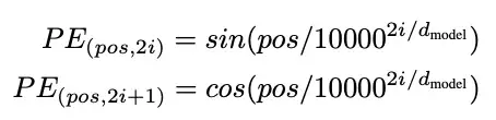
포지션 인코딩은 입력 데이터의 순서를 기억할 수 있는 순환 네트워크가 없기 때문에, 시퀀스의 모든 단어/부분에 상대적인 위치를 계산하는 방식이다. 이러한 위치는 각 단어의 포함된 표현(n차원 벡터)에 추가된다. 보통, 이 방식은 다음의 sin, cos함수를 통해 토큰이 텍스트에서 사용된 i번째 위치 벡터를 계산한다.

포지션 인코딩 함수

사용 예시

사용 예시를 간단히 확인해 본다. 이를 위해 아래 링크를 참고하도록 한다.

• Text Transformer: BERT, GPT-3같은 문서 종류 분류, 번역, 작문, 챗봇, 주가예측, 작사 등

• Vision Transformer (ViT): 객체 분류, 탐지, 세그먼테이션, 텍스트 캡션 생성 등

SegFormer: Simple and Efficient Design for Semantic Segmentation with Transformers

• Point cloud Transformer (PCT): 점군 생성, 분류, 세그먼테이션 등

Point Transformer

PCT using BERT(Bidirectional Encoder Representations from Transformers)

사용 방법

파이토치 등 유명한 딥러닝 라이브러리는 이미 트랜스포머 모듈을 구현해 두고 있다. 이를 이용해, 예측, 분류, 세그먼테이션 등을 다양한 데이터셋(텍스트, 이미지, 점군, 기하 벡터 등)에 대해 수행할 수 있다.

• PyTorch, LANGUAGE MODELING WITH NN.TRANSFORMER AND TORCHTEXT

이 예제의 목표는 다음과 같은 입력에 대한 출력을 예측하는 것이다. 참고로, 데이터의 종류는 텍스트이지만, 수치화할 수 있다면, 이미지, 소리 등 종류에 구애받지 않는다.

이 예제는 학습 데이터를 Wikitext-2(https://github.com/pytorch/data)를 사용한다. 미리 다운로드 받아 둔다. 어휘의 토큰은 센서로 수치화되어 학습될 것이다. 이 텍스트 시퀀스는 batchify()란 함수에 의해, batch_size 수의 컬럼으로 변환된다. 예를 들어, 26개 알파벳 시퀀스를 batch_size=4로 정의할 때 다음과 같은 6개의 4개의 시퀀스로 변환된다. 

파이토치 구현 코드는 다음과 같다.

import math

from typing import Tuple

import torch

from torch import nn, Tensor

import torch.nn.functional as F

from torch.nn import TransformerEncoder, TransformerEncoderLayer  # 트랜스포머 모듈 

from torch.utils.data import dataset

class TransformerModel(nn.Module):

    def __init__(self, ntoken: int, d_model: int, nhead: int, d_hid: int,

                 nlayers: int, dropout: float = 0.5):

        super().__init__()

        self.model_type = 'Transformer'

        self.pos_encoder = PositionalEncoding(d_model, dropout)  # 포지션 인코딩

        encoder_layers = TransformerEncoderLayer(d_model, nhead, d_hid, dropout) # 트랜스포머 인코딩 레이어

        self.transformer_encoder = TransformerEncoder(encoder_layers, nlayers)  # 트랜스포머 레이어

        self.encoder = nn.Embedding(ntoken, d_model)  # 임베딩

        self.d_model = d_model

        self.decoder = nn.Linear(d_model, ntoken)

        self.init_weights()

    def init_weights(self) -> None:

        initrange = 0.1

        self.encoder.weight.data.uniform_(-initrange, initrange)

        self.decoder.bias.data.zero_()

        self.decoder.weight.data.uniform_(-initrange, initrange)

    def forward(self, src: Tensor, src_mask: Tensor) -> Tensor:

        """

        Args:

            src: Tensor, shape [seq_len, batch_size]

            src_mask: Tensor, shape [seq_len, seq_len]

        Returns:

            output Tensor of shape [seq_len, batch_size, ntoken]

        """

        src = self.encoder(src) * math.sqrt(self.d_model) # 임베딩 x 어텐션

        src = self.pos_encoder(src)  # 위치인코딩

        output = self.transformer_encoder(src, src_mask) # 트랜스포머

        output = self.decoder(output) # linear

        return output

def generate_square_subsequent_mask(sz: int) -> Tensor:  # 어텐션 마스크 처리

    """Generates an upper-triangular matrix of -inf, with zeros on diag."""

    return torch.triu(torch.ones(sz, sz) * float('-inf'), diagonal=1)

포지션 인코딩은 다음과 같다. 

class PositionalEncoding(nn.Module):

    def __init__(self, d_model: int, dropout: float = 0.1, max_len: int = 5000):

        super().__init__()

        self.dropout = nn.Dropout(p=dropout)

        position = torch.arange(max_len).unsqueeze(1)

        div_term = torch.exp(torch.arange(0, d_model, 2) * (-math.log(10000.0) / d_model))

        pe = torch.zeros(max_len, 1, d_model)

        pe[:, 0, 0::2] = torch.sin(position * div_term)

        pe[:, 0, 1::2] = torch.cos(position * div_term)

        self.register_buffer('pe', pe)

    def forward(self, x: Tensor) -> Tensor:

        """

        Args:

            x: Tensor, shape [seq_len, batch_size, embedding_dim]

        """

        x = x + self.pe[:x.size(0)]

        return self.dropout(x)

입력 텍스트를 배치 단위로 변환하는 코드는 다음과 같다. 

from torchtext.datasets import WikiText2   # 학습 데이터

from torchtext.data.utils import get_tokenizer

from torchtext.vocab import build_vocab_from_iterator

train_iter = WikiText2(split='train')

tokenizer = get_tokenizer('basic_english')   # 기본영어 텍스트에서 토큰 획득

vocab = build_vocab_from_iterator(map(tokenizer, train_iter), specials=['<unk>'])

vocab.set_default_index(vocab['<unk>'])

def data_process(raw_text_iter: dataset.IterableDataset) -> Tensor:

    # 입력 텍스트를 토큰화해 수치 텐서로 변환함

    data = [torch.tensor(vocab(tokenizer(item)), dtype=torch.long) for item in raw_text_iter]

    return torch.cat(tuple(filter(lambda t: t.numel() > 0, data)))

# 학습, 검증 및 테스트 데이터를 텐서로 변환

# so we have to create it again

train_iter, val_iter, test_iter = WikiText2()

train_data = data_process(train_iter)

val_data = data_process(val_iter)

test_data = data_process(test_iter)

device = torch.device('cuda' if torch.cuda.is_available() else 'cpu')

def batchify(data: Tensor, bsz: int) -> Tensor:

    # 주어진 배치개수 만큼 배치 데이터 생성

    seq_len = data.size(0) // bsz

    data = data[:seq_len * bsz]

    data = data.view(bsz, seq_len).t().contiguous()

    return data.to(device)

batch_size = 20

eval_batch_size = 10

train_data = batchify(train_data, batch_size)  # 배치데이터 생성. shape [seq_len, batch_size]

val_data = batchify(val_data, eval_batch_size)

test_data = batchify(test_data, eval_batch_size)

이제, 입력에 대한 출력(라벨) 데이터를 생성한다.

bptt = 35

def get_batch(source: Tensor, i: int) -> Tuple[Tensor, Tensor]:

    seq_len = min(bptt, len(source) - 1 - i)

    data = source[i:i+seq_len]

    target = source[i+1:i+1+seq_len].reshape(-1)

    return data, target

이제 하이퍼파라메터를 조정한다. 

ntokens = len(vocab) # 단어 사전(어휘집)의 크기

emsize = 200 # 임베딩 차원

d_hid = 200 # nn.TransformerEncoder 에서 피드포워드 네트워크(feedforward network) 모델의 차원

nlayers = 2 # nn.TransformerEncoder 내부의 nn.TransformerEncoderLayer 개수

nhead = 2 # nn.MultiheadAttention의 헤드 개수

dropout = 0.2 # 드랍아웃(dropout) 확률

model = TransformerModel(ntokens, emsize, nhead, d_hid, nlayers, dropout).to(device)

모델을 학습한다. 손실함수는 CrossEntropyLoss로 SGD 함수를 사용하고, step learning rate를 설정하며, nn.utils.clip_grad_norm_ 함수를 사용해 기울이가 발산하지 않도록 한다.

import copy

import time

criterion = nn.CrossEntropyLoss()

lr = 5.0  # 학습률(learning rate)

optimizer = torch.optim.SGD(model.parameters(), lr=lr)

scheduler = torch.optim.lr_scheduler.StepLR(optimizer, 1.0, gamma=0.95)

def train(model: nn.Module) -> None:

    model.train()  # 학습 모드 시작

    total_loss = 0.

    log_interval = 200

    start_time = time.time()

    src_mask = generate_square_subsequent_mask(bptt).to(device)

    num_batches = len(train_data) // bptt

    for batch, i in enumerate(range(0, train_data.size(0) - 1, bptt)):

        data, targets = get_batch(train_data, i)

        seq_len = data.size(0)

        if seq_len != bptt:  # 마지막 배치에만 적용

            src_mask = src_mask[:seq_len, :seq_len]

        output = model(data, src_mask)

        loss = criterion(output.view(-1, ntokens), targets)  # 손실함수 계산

        optimizer.zero_grad()

        loss.backward()  # 가중치 업데이트

        torch.nn.utils.clip_grad_norm_(model.parameters(), 0.5)

        optimizer.step()

        total_loss += loss.item()

        if batch % log_interval == 0 and batch > 0:

            lr = scheduler.get_last_lr()[0]

            ms_per_batch = (time.time() - start_time) * 1000 / log_interval

            cur_loss = total_loss / log_interval

            ppl = math.exp(cur_loss)

            print(f'| epoch {epoch:3d} | {batch:5d}/{num_batches:5d} batches | '

                  f'lr {lr:02.2f} | ms/batch {ms_per_batch:5.2f} | '

                  f'loss {cur_loss:5.2f} | ppl {ppl:8.2f}')

            total_loss = 0

            start_time = time.time()

def evaluate(model: nn.Module, eval_data: Tensor) -> float:

    model.eval()  # 평가 모드 시작

    total_loss = 0.

    src_mask = generate_square_subsequent_mask(bptt).to(device)

    with torch.no_grad():

        for i in range(0, eval_data.size(0) - 1, bptt):

            data, targets = get_batch(eval_data, i)

            seq_len = data.size(0)

            if seq_len != bptt:

                src_mask = src_mask[:seq_len, :seq_len]

            output = model(data, src_mask)

            output_flat = output.view(-1, ntokens)

            total_loss += seq_len * criterion(output_flat, targets).item()

    return total_loss / (len(eval_data) - 1)

이제 Epoch 마다 학습 및 평가를 수행하는 train(), evaluate()함수를 호출한다.

best_val_loss = float('inf')

epochs = 3

best_model = None

for epoch in range(1, epochs + 1):

    epoch_start_time = time.time()

    train(model)

    val_loss = evaluate(model, val_data)

    val_ppl = math.exp(val_loss)

    elapsed = time.time() - epoch_start_time

    print('-' * 89)

    print(f'| end of epoch {epoch:3d} | time: {elapsed:5.2f}s | '

          f'valid loss {val_loss:5.2f} | valid ppl {val_ppl:8.2f}')

    print('-' * 89)

    if val_loss < best_val_loss:

        best_val_loss = val_loss

        best_model = copy.deepcopy(model)

    scheduler.step()

그 결과는 다음과 같다.

학습 결과를 다음 코드로 평가한다.

test_loss = evaluate(best_model, test_data)

test_ppl = math.exp(test_loss)

print('=' * 89)

print(f'| End of training | test loss {test_loss:5.2f} | '

      f'test ppl {test_ppl:8.2f}')

print('=' * 89)

마무리

트랜스포머의 어텐션 메커니즘을 응용하면, 학습 데이터의 전역적인 특징을 고려한, 데이터 분류, 예측, 탐지, 생성이 가능하다. 임베딩 기법을 이용해, 영상 등 비정형적인 데이터를 학습데이터로 활용할 수 있어, 그 활용도가 더욱 높아질 것이다.

레퍼런스

• Transformer Wiki
• What is Transfomer
• Transformer Illustration
• List Transformer
• Transformer Chatbot (wiki)
• Attention, self-attention, transformer (2nd)
• Build your own Transformer from scratch using Pytorch | by Arjun Sarkar | Towards Data Science
• A complete Hugging Face tutorial: how to build and train a vision transformer | AI Summer (theaisummer.com)
• Fast Transformer Inference with Better Transformer — PyTorch Tutorials 2.1.1+cu121 documentation

pyLiDAR-SLAM 사용하기

이 글은 라이다 스캔을 통해 얻은 데이터를 이용해 실시간 SLAM 처리하는 알고리즘을 파이썬으로 라이브러리화한 pyLiDAR-SLAM 사용 방법을 간략히 공유한다.

설치

우분투 리눅스 운영체제에서 실행하므로, 아래 링크 등을 참고해 실행 환경을 미리 준비한다.

• 우분투 리눅스 운영체제 설치

다음 메뉴얼을 참고해 설치한다. 의존하고 있는 패키지 pycp_icp (python3 binding 필요), pyviz3d, opencv, g2o, open3d 모두 메뉴얼을 참고해 설치한다.

• Install pyLiDAR

설치 시 여러가지 에러가 발생한다. 아래를 참고해 해결해 나간다.

• 설치하기 전에 패키지 의존 에러가 발생할 수 있으므로, 가상환경을 터미널에서 아래와 같이 활성화한다. 

pip install --force-reinstall virtualenv

pip3 install --force-reinstall virtualenv

virtualenv venv_pylidar

source ./venv_pylidar/bin/activate 

• cmake 처리 시 virtualenv를 제대로 인식해 python3를 못찾을 수 있다. 이 경우, 아래와 같이 경로를 지정해 준다.

cmake .. -DPYTHON_EXECUTABLE=/home/ktw/Projects/pyLiDAR-SLAM/venv_pylidar/bin/python3 

• 의존 패키지가 사용하는 github 소스코드 빌드 처리를 위해, github 로그인을 위한 계정, RSA 암호 키 등을 아래 링크를 참고해 터미널에서 설정한다.

• First time git setting

• 몇몇 의존 패키지에서 사용하는 라이브러리에 에러가 발생할 수 있다. 아래는 이와 관련해 설치한 라이브러리이다.

pip install hydra-core --upgrade

pip install pygame 
pip install PyOpenGL

pip install PyOpenGL-accelerate

pip install omegaconf 

• Eigen 패키지에서 버전 차이로 인해 Quaternion에서 컴파일 에러가 발생할 수 있다. 아래와 같이 처리한다.

/* .def("x", (NonConstCoeffReturnType (Eigen::Quaterniond::*) () const) &Eigen::Quaterniond::x())

        .def("y", (NonConstCoeffReturnType (Eigen::Quaterniond::*) () const) &Eigen::Quaterniond::y())

        .def("z", (NonConstCoeffReturnType (Eigen::Quaterniond::*) () const) &Eigen::Quaterniond::z())

        .def("w", (NonConstCoeffReturnType (Eigen::Quaterniond::*) () const) &Eigen::Quaterniond::w()) */

설치가 끝나면 다음과 같다.

사용

사용 방법을 확인하기 위해 예제 데이터를 프로젝트 폴더에 다운받고, 다음을 실행한다.

python3 run.py -m num_workers=1 slam/initialization=NI slam/preprocessing=none slam/odometry=ct_icp_robust_shaky, icp_odometry slam.odometry.viz_debug=True slam/loop_closure=none slam/backend=none dataset=rosbag dataset.main_topic=horizontal_laser_3d dataset.accumulate_scans=True  dataset.file_path=./b3-2016-04-05-15-51-36.bag hydra.run.dir=./TEST_DOC

혹은 아래와 같이 실행할 수도 있다.

python3 run.py num_workers=1 slam/initialization=NI slam/preprocessing=none slam/odometry=ct_icp_robust_shaky slam.odometry.viz_debug=True slam/loop_closure=none slam/backend=none dataset=rosbag dataset.main_topic=horizontal_laser_3d dataset.accumulate_scans=True  dataset.file_path=./b3-2016-04-05-15-51-36.bag hydra.run.dir=./TEST_DOC

참고로, 이 프로그램의 형식은 다음과 같다.

python3 run.py num_workers=1 /  # The number of process workers to load the dataset

    slam/initialization=NI /              # The initialization (NI=No Initialization / CV=Constant Velocity)

    slam/preprocessing=grid_sample /    # Preprocessing on the point clouds

    slam/odometry=icp_odometry /        # The Odometry algorithm

    slam.odometry.viz_debug=True /      # Whether to launch the visualization of the odometry

    slam/loop_closure=none /            # The loop closure algorithm selected (none by default)

    slam/backend=none /                   # The backend algorithm (none by default)

    dataset=rosbag /                           # The dataset selected (a simple rosbag here)

    dataset.main_topic=horizontal_laser_3d /    # The pointcloud topic of the rosbag 

    dataset.accumulate_scans=True /                 # Whether to accumulate multiple messages  

    dataset.file_path=./b3-2016-04-05-15-51-36.bag /    #  The path to the rosbag file 

    hydra.run.dir=./TEST_DOC        #  The log directory where the trajectory will be saved

실행 시 다음과 같이 hydra 패키지에서 에러가 발생할 수 있다.

사용 후에는 반듯이 가상환경을 빠져나와 패키지 설치 환경이 오염되지 않도록 한다.

deactivate

레퍼런스

• pyLiDAR-SLAM

임베디드보드 및 웹 기반 딥러닝 모델 실행을 위한 Tensorflow Lite 사용하기

이 글은 임베디드보드에서 딥러닝 모델 실행을 위한 Tensorflow Lite 및 Tensorflow JS (TFJS) 사용 방법을 간략히 공유한다. 이 내용은 딥러닝 기반 에지(Edge) 컴퓨팅 구현이나 가벼운 웹브라우저 기반 딥러닝 응용 서비스 개발에 도움이 된다. 

머리말

텐서플로우 라이트와 TFJS는 개발자가 모바일, 임베디드 장치, IoT, 웹브라우저에서 딥러닝 모델을 실행할 수 있도록, 모델을 최적화하는 도구이다. 특징은 다음과 같다.

• 특정 장치에서 실행되도록 딥러닝 모델을 최적화함. 모델 크기 및 전력 소모 축소.
• 다중 플랫폼 지원. 안드로이드, iOS, 임베디드, Javascript 웹브라우저, 리눅스 등.
• 하드웨어 가속 지원.

실행 개념

텐서플로우 라이트 실행 환경은 목표하는 플랫폼에 따라 다르다. 예를 들어, 임베디드 중 아두이노에서 개발한다면, 이에 대한 라이브러리가 준비되어 있어서, 이를 사용하면 된다. 

• Arduino Nano 33 BLE보드와 TinyML 기반 딥러닝 처리 방법 및 사용기

사용은 매우 쉬운 편인데, 기존 텐서플로우 딥러닝 모델을 작업한 후, 라이트버전으로 변환하면 된다. 변환함수를 당연히 제공하고, 변환시 모델의 실수 데이터 형식은 정수로 자동 변환된다. 참고로, 정수는 실수보다 크기가 4배 적고, 처리 속도는 훨씬 빠르다. 이런 이유로, GPU가 없는 컴퓨터에서도 딥러닝 모델을 빠르게 실행시킬 수 있다. 물론, 이 변환 후에는 실수형 연산 함수는 사용할 수 없다(API 호환성). 몇몇 플랫폼은 연산가속칩이 있다. 라이트는 이 기능을 이용할 수 있다.

변환된 모델은 FlatBuffers형식인 .tflite 확장자인 파일로 저장된다. 이 파일은 메타데이터를 포함할 수 있고, 이 경우, 텐서플로우 라이트 API를 사용하지 않고, 파일 로딩 후 바로 실행할 수 있다.

이제, 각 실행환경에서 사용방법을 확인해 본다.

CoLab기반 딥러닝 모델 생성 및 최적화

CoLab은 구글에서 지원하는 머신러닝 협업 및 연구용 플랫폼으로 대부분 기능이 무료이다. 

• 구글 코랩으로 쉽게 딥러닝해 보기

여기서는 CoLab을 사용해 MNIST를 이용해 CNN모델을 만들고, 이를 라이트버전으로 처리해본다. 직접 실행은 여기를 참고한다. 

다음 코드를 CoLab에 입력해 실행해 본다. 최적화하는 부분인 TFLiteConverter 함수 사용만 다르고, 나머지는 일반적인 텐서플로우 코딩과 같다는 것을 알 수 있다.

# 라이브러리 로딩

import logging

logging.getLogger("tensorflow").setLevel(logging.DEBUG)

import tensorflow as tf

from tensorflow import keras

import numpy as np

import pathlib

# MNIST 로딩

mnist = keras.datasets.mnist

(train_images, train_labels), (test_images, test_labels) = mnist.load_data()

# 입력 이미지 정규화 

train_images = train_images / 255.0

test_images = test_images / 255.0

# 딥러닝 모델 구조 정의

model = keras.Sequential([

  keras.layers.InputLayer(input_shape=(28, 28)),

  keras.layers.Reshape(target_shape=(28, 28, 1)),

  keras.layers.Conv2D(filters=12, kernel_size=(3, 3), activation=tf.nn.relu),

  keras.layers.MaxPooling2D(pool_size=(2, 2)),

  keras.layers.Flatten(),

  keras.layers.Dense(10)

])

# 필기체 이미지 분류 모델 학습. 1세대만 처리.

model.compile(optimizer='adam',

              loss=keras.losses.SparseCategoricalCrossentropy(from_logits=True),

              metrics=['accuracy'])

model.fit(

  train_images,

  train_labels,

  epochs=1,

  validation_data=(test_images, test_labels)

)

# TFLite버전으로 모델 변환

converter = tf.lite.TFLiteConverter.from_keras_model(model)

tflite_model = converter.convert()

tflite_models_dir = pathlib.Path("/tmp/mnist_tflite_models/") # 폴더 생성

tflite_models_dir.mkdir(exist_ok=True, parents=True)

tflite_model_file = tflite_models_dir/"mnist_model.tflite"

tflite_model_file.write_bytes(tflite_model)  # TFLite 파일로 파일 저장

# 최적화 옵션 켜서 모델 저장

converter.optimizations = [tf.lite.Optimize.DEFAULT]

tflite_quant_model = converter.convert()

tflite_model_quant_file = tflite_models_dir/"mnist_model_quant.tflite"

tflite_model_quant_file.write_bytes(tflite_quant_model) 

!ls -lh {tflite_models_dir}  # CoLab 확인해 보면, 실제 최적화된 모델은 기존 모델의 1/4임

이제 저장된 TFLite 모델을 실행해보자. 아래 코드를 CoLab에 입력해 실행해 본다.

interpreter = tf.lite.Interpreter(model_path=str(tflite_model_file))  

interpreter.allocate_tensors()            # 최적화 안된 TFLite

interpreter_quant = tf.lite.Interpreter(model_path=str(tflite_model_quant_file))

interpreter_quant.allocate_tensors()   # 최적화된 TFLite

test_image = np.expand_dims(test_images[0], axis=0).astype(np.float32)  # 첫번째 테스트 이미지

input_index = interpreter.get_input_details()[0]["index"]

output_index = interpreter.get_output_details()[0]["index"]

interpreter.set_tensor(input_index, test_image)

interpreter.invoke()  # 모델 실행

predictions = interpreter.get_tensor(output_index)  # 예측 결과 얻기

import matplotlib.pylab as plt

plt.imshow(test_images[0])

template = "True:{true}, predicted:{predict}"

_ = plt.title(template.format(true= str(test_labels[0]),

                              predict=str(np.argmax(predictions[0]))))

plt.grid(False)

TFLite 모델 정확도를 평가해 보자. 아래 코드를 입력해 본다.

# TF Lite 모델 평가용 유틸리티 함수

def evaluate_model(interpreter):

  input_index = interpreter.get_input_details()[0]["index"]

  output_index = interpreter.get_output_details()[0]["index"]

  # 테스트 데이터셋 예측

  prediction_digits = []

  for test_image in test_images:

    # 전처리는 배치로 32비트 실수를 모델 데이터 형식으로 변환하도록 함

    test_image = np.expand_dims(test_image, axis=0).astype(np.float32)

    interpreter.set_tensor(input_index, test_image)

    # 모델 예측 실행

    interpreter.invoke()

    # 후처리는 가장 높은 정확도 probability 클래스를 찾음

    output = interpreter.tensor(output_index)

    digit = np.argmax(output()[0])

    prediction_digits.append(digit)

  # 그라운드 참값과 차이 비교

  accurate_count = 0

  for index in range(len(prediction_digits)):

    if prediction_digits[index] == test_labels[index]:

      accurate_count += 1

  accuracy = accurate_count * 1.0 / len(prediction_digits)

  return accuracy

print(evaluate_model(interpreter))

print(evaluate_model(interpreter_quant))

실제 평가해 보면, 각각 0.9671, 0.9669로 별 차이가 없다.

Javascript 웹 기반 딥러닝 실행

자바스크립트 웹 기반 딥러닝 실행을 위해, TFJS 라이브러리를 사용한다. 우선, 자바스크립트 node.js 를 이용해 딥러닝 모델을 작성한 후 실행해 본다(참고 - 여기와 TFJS Task API).

우선 터미널에서 아래 명령을 실행한다. 

mkdir tfjs

cd tfjs

npm install @tensorflow/tfjs-node

npm install @tensorflow/tfjs-node-gpu

demo.js 코드를 아래와 같이 작성한다.

const tf = require('@tensorflow/tfjs');  // tfjs 임포트

const model = tf.sequential();               // 시퀀스 모델 생성

model.add(tf.layers.dense({units: 100, activation: 'relu', inputShape: [10]}));    

model.add(tf.layers.dense({units: 1, activation: 'linear'})); 

model.compile({optimizer: 'sgd', loss: 'meanSquaredError'});

const xs = tf.randomNormal ([100, 10]);   // 학습 입력 데이터

const ys = tf.randomNormal ([100, 1]);     // 결과 라벨 데이터

model.fit (xs, ys, 

{epochs : 100, 

callbacks : {onEpochEnd : (epoch, log) => console.log ( epoch + " = " + log.loss )} 

});  // 학습

터미널에서 아래 명령을 실행한다. 학습이 잘 되는 것을 확인할 수 있다.

node demo.js

웹브라우저에서 딥러닝 모델을 사용하는 방법을 확인해 보기 위해, 우분투 리눅스 터미널에서 아래 명령을 실행하고 관련 예제를 다운로드한다.

git clone https://github.com/tensorflow/tfjs-models

cd tfjs-models

테스트할 딥러닝 모델을 다운로드 설치한다. 기타 필요한 모델은 여기서 확인한다.

npm i @tensorflow-models/coco-ssd

npm i @tensorflow-models/mobilenet

npm i @tensorflow-models/deeplab

yarn 프로젝트 관리 및 빌드 도구를 설치한다. yarn에 대한 설명은 여기를 참고하라.

curl -sS https://dl.yarnpkg.com/debian/pubkey.gpg | sudo apt-key add -

echo "deb https://dl.yarnpkg.com/debian/ stable main" | sudo tee /etc/apt/sources.list.d/yarn.list

sudo apt-get update

sudo apt-get install yarn

sudo npm install --global cross-env

패키지를 빌드한다.

yarn

yarn presubmit

설치된 딥러닝 모델 테스트를 위해 아래 명령을 실행한다.

cd coco-ssd

cd demo

yarn

yarn build-deps

yarn run

watch

웹서버가 실행되었다면, http://localhost:1234/ 에서 결과를 확인해 본다. 다음과 같이 정상적으로 웹브라우저에서 딥러닝이 실행되는 것을 확인할 수 있다.

COCO-SSD 모델의 demo 폴더 구조는 다음과 같다. 

주요 코드는 다음과 같다. 아래 index.html에서 웹화면 레이아웃을 정의한다.

 

<!doctype html>

<html>

<body>

  <h1>TensorFlow.js Object Detection</h1>

  <select id='base_model'>

    <option value="lite_mobilenet_v2">SSD Lite Mobilenet V2</option>

    <option value="mobilenet_v1">SSD Mobilenet v1</option>

    <option value="mobilenet_v2">SSD Mobilenet v2</option>

  </select>

  <button type="button" id="run">Run</button>

  <button type="button" id="toggle">Toggle Image</button>

  <div>

    <img id="image" />

    <canvas id="canvas" width="600" height="399"></canvas>

  </div>

</body>

<script src="index.js"></script>

</html>

실제 동작코드는 index.js 자바스크립트에 코딩된다.

import '@tensorflow/tfjs-backend-cpu';      // tfjs 패키지 임포트

import '@tensorflow/tfjs-backend-webgl';

import * as cocoSsd from '@tensorflow-models/coco-ssd';  // coco-ssd 모델 임포트

import imageURL from './image1.jpg';      // 폴더에 정의된 이미지 임포트

import image2URL from './image2.jpg';

let modelPromise;

window.onload = () => modelPromise = cocoSsd.load();

const button = document.getElementById('toggle');   // 토글버튼 클릭시 이미지 교체

button.onclick = () => {

  image.src = image.src.endsWith(imageURL) ? image2URL : imageURL;

};

const select = document.getElementById('base_model');

select.onchange = async (event) => {

  const model = await modelPromise;   // 모델 선택 변경 시 모델 재로딩

  model.dispose();

  modelPromise = cocoSsd.load(

      {base: event.srcElement.options[event.srcElement.selectedIndex].value});

};

const image = document.getElementById('image');

image.src = imageURL;

const runButton = document.getElementById('run');

runButton.onclick = async () => {   // 실행 버튼 클릭시, 이미지 입력 후 모델 예측 실행

  const model = await modelPromise;

  console.log('model loaded');

  console.time('predict1');

  const result = await model.detect(image);

  console.timeEnd('predict1');

  const c = document.getElementById('canvas');  // 캔버스 요소 획득 후 이미지 렌더링

  const context = c.getContext('2d');

  context.drawImage(image, 0, 0);

  context.font = '10px Arial';

  console.log('number of detections: ', result.length);   // 예측 결과 이미지 및 라벨 렌더링

  for (let i = 0; i < result.length; i++) {

    context.beginPath();

    context.rect(...result[i].bbox);

    context.lineWidth = 1;

    context.strokeStyle = 'green';

    context.fillStyle = 'green';

    context.stroke();

    context.fillText(

        result[i].score.toFixed(3) + ' ' + result[i].class, result[i].bbox[0],

        result[i].bbox[1] > 10 ? result[i].bbox[1] - 5 : 10);

  }

};

TFJS 라이브러리가 대부분의 딥러닝 모델 사용 과정을 캡슐화하여, 실제 사용되는 함수는 그리 많지 않음을 알 수 있다. 직접 모델을 훈련하고, 웹에서 서비스를 제공하기 위한 목적으로 아래 Tutorial을 참고할 수 있다.

• Deploying a Simple Machine Learning Model into a WebApp using TensorFlow.js

마무리

TFLite를 이용하면, GPU가 없는 다양한 플랫폼에서 적은 메모리와 정확도 손실로 딥러닝 모델을 실행할 수 있다.

레퍼런스

• 텐서플로우 라이드 시작하기
• 엔비디아 스트림
• Tensorflow.js 사용하기 (webcam)
• YARN installation

CNN 딥러닝 파라메터에 따른 예측 정확도 변화 확인

이 글은 CNN(Convolution Neural Network) 딥러닝 파라메터에 따른 예측 정확도 변화 확인 결과를 간략히 정리한다. 딥러닝 모델은 파라메터가 어떻게 되느냐에 따라 정확도가 달라진다. 얼마나 차이가 나는지를 확인해 보기 위해, CNN 모델을 정의하고, 파라메터를 조정해 본다. 

기본 모델 정의

기본 모델은 다음과 같다. 이 모델은 주어진 이미지를 2개의 클래스로 구분한다. 

# Our input feature map is 150x150x3: 150x150 for the image pixels, and 3 for

# the three color channels: R, G, and B

img_input = layers.Input(shape=(150, 150, 3))

x = layers.Conv2D(16, 3, activation='relu')(img_input)

x = layers.MaxPooling2D(2)(x)

x = layers.Conv2D(32, 3, activation='relu')(x)

x = layers.MaxPooling2D(2)(x)

x = layers.Conv2D(64, 3, activation='relu')(x)

x = layers.MaxPooling2D(2)(x)

x = layers.Flatten()(x)

x = layers.Dense(512, activation='relu')(x)

output = layers.Dense(1, activation='sigmoid')(x)

model = Model(img_input, output)

실제 학습은 아래 CoLab으로 진행해본다.

• CoLab classification example

대표적인 CNN 분류 예시

모델 파라메터 조정 결과

CNN 커널 크기와 계층수를 변화시켜보도록 한다. 모델 파라메터를 조정한 결과는 다음과 같다.

커널 3계층 표준

커널 크기 증가1

커널 크기 증가2

커널 2계층

커널 4계층

결론

결과는 CNN 필터를 배수로 증가시켜가면서 모델을 추가했을 때 정확도가 높았다. 또한, 커널 계층을 삭제하거나 증가할때 정확도나 손실은 좋아지지 않았다. 이런 파라메터는 입력 데이터 특성 등에 따라 조정해 나가야 한다. 참고로, 이런 노가다는 AutoML같은 최적 모델 선택 도구를 통해 줄일 수 있다.

레퍼런스

• 텐서플로우 라이트 저장
• AutoML